# Encode Wiki full corpus
Content version: d505714a5a686d22c08eede79a428587acaa46b8
# AV1 Encoding for Dummies
Canonical URL: https://encode.wiki/articles/av1-encoding-for-dummies/
Collection: articles
Status: needs-review
License: CC BY-SA 4.0
Checksum: 17a1eafe2fa5bc78e692d6e62111eb65349194a12c864bdea4eb0cb3c87c7ea1
This guide will show you how to encode in AV1 the *right* and *optimal* way. Yes, you using standalone ``libaom``, ``libsvtav1``, and ``librav1e`` from FFmpeg or even piping ``yuv4mpeg`` into **mainline** aomenc are all unoptimal.
> **Danger — Outdated Information.**
>
> While a lot of the information presented in this guide is still relevant and correct, the AV1 ecosystem has changed dramatically since this guide's inception which has demanded a rewrite. Please see the [AV1 for Dummies](/articles/av1-for-dummies/) blog post for more information.

In this guide, we'll be installing Av1an for chunked encoding and infinite threading, because the current state of AV1 encoders, except for [SVT-AV1](/tools/software-encoders/svt-av1/), unfortunately lacks threading and will only use very low amount of cores, which hampers speeds. The only caveat to this approach is **RAM consumption**, encoding 2160p (4K) with [aomenc](/tools/software-encoders/aomenc/) with 4 workers could take upwards of **16GB** of RAM! So do keep this in mind.
## Installing the Tools
Given all of the different operating systems that people use on a day to day basis and the various different encoding workflows that exist, there are a number of ways to do this.
**Jump to**: [Windows](#microsoft-windows) | [macOS](#macos) | [Linux](#linux)
## Microsoft Windows
### The GUI Way
1. Install [NMKODER](https://github.com/n00mkrad/nmkoder) which is a GUI front-end to av1an with all dependencies installed.
2. You're done, you can skip to the encoding part
> **Danger — Almost abandonware.**
>
> Since Nmkoder already ships everything by default and its last release was 29th March 2022. You need to manually update all encoders and tools to get better encoding speeds. Missing out on updates will result in your encodes being sub-optimal.
### The WSL2 Way
*(Recommended)*
If you're not already familiar with WSL2, the The Windows Subsystem for Linux (WSL) is a feature of the Windows operating system that allows you to run a Linux file system, along with Linux command-line tools and GUI apps, directly on Windows. This lets Linux distributions run on bare metal without managing any virtual machines, so encoding performance is very good.
The easiest way to encode with WSL2 is to use [rAV1ator CLI](/tools/utilities/rav1ator-cli/), an interactive TUI for [Av1an](/tools/utilities/av1an/). An ArchWSL2 installation tutorial is provided [here](/tools/utilities/rav1ator-cli/#windows).
### The Automated Way
There is now a batch script for automating the install process, which can be found [here](https://github.com/Hishiro64/av1an-win-script). The instructions are in the README file.
> **Caution — The script will download outdated version encoders and tools such as `aom-av1-psy` and MKVToolNix v76.0, if you are fine with these you can proceed..**
>
>
### The Manual Way
1. Install **Python 3.10.x, this will change so consult from the** [Vapoursynth website](http://www.vapoursynth.com/doc/installation.html) **if you're reading this from the future** from [here](https://www.python.org/downloads/windows/) and select "Windows Installer 64-bit". Upon installation check the tick for adding Python to PATH like so
)
2. Download and install Vapoursynth from [here](https://github.com/vapoursynth/vapoursynth/releases) and select "VapourSynth64-RXX.exe"
3. Open the terminal and type ``vsrepo.py install lsmas ffms2`` to install some plugins for Av1an to work.
4. Download MKVToolNix from [here](https://mkvtoolnix.download/downloads.html#windows), select "mkvtoolnix-64bit-XX.X.X-setup.exe", and install **(Also available on winget!)**
5. Download Av1an from [here](https://github.com/master-of-zen/Av1an/releases) (SELECT LATEST AND CLICK THE "ASSETS" DROPDOWN)
6. Download **shared libraries** FFmpeg from [gyan.dev](https://www.gyan.dev/ffmpeg/builds)
7. Download or build the Aomenc fork [aom-av1-lavish](https://github.com/Clybius/aom-av1-lavish/tree/Endless_Merging), which has features such as different defaults, tunes, and optimizations. The Windows binary linked by the original September 2023 guide is no longer available; check the project or AV1 community channels for a current build.
> **Info — If you opt to compile aomenc yourself, you can view the instructions on how to do that [here](/tools/software-encoders/aomenc/#installation)..**
>
>
8. Move Av1an, FFmpeg **(Including the FFmpeg DLLs)**, and aomenc to somewhere preferable, eg ``C:\Encoding``.
9. Add the folder **AND MKVTOOLNIX INSTALLATION FOLDER** to the [Windows PATH environment](https://www.maketecheasier.com/what-is-the-windows-path/).
## macOS
macOS is very similar to Linux, although there aren't any GUI tools for AV1 encoding that I can comfortably recommend.
**Homebrew + Macports for Av1an + rav1e:**
*Note that some commands may have to be run with `sudo`, which I won't explicitly include for security reasons.*
Installing the Homebrew package manager is a well documented process at this point:
```bash
/bin/bash -c "$(curl -fsSL https://raw.githubusercontent.com/Homebrew/install/HEAD/install.sh)"
```
As is installing MacPorts. Install the relevent `.pkg` for your macOS version from the MacPorts Project website:
[www.macports.org/install.php](https://www.macports.org/install.php)
Now, you can run the following commands:
```bash
brew update && brew upgrade
brew install rav1e aom mkvtoolnix ffmpeg
# Usually you must run MacPorts commands for package installations as root
port upgrade outdated
port install av1an
```
This is the easiest way to get everything set up & working to produce AV1 video with `rav1e` or mainline `aomenc` & Av1an. You can check that things are installed by running the following commands & parsing their output:
```bash
% av1an --version
av1an 0.4.1-unstable (rev e10880d) (Release)
* Compiler
rustc 1.70.0 (LLVM 16.0)
* Target Triple
aarch64-apple-darwin
* Date Info
Commit Date: 2023-06-25
* VapourSynth Plugins
systems.innocent.lsmas : Not found
com.vapoursynth.ffms2 : Not found
```
```bash
% rav1e --version | grep "release" -C 1
rav1e 0.6.6 () (release)
rustc 1.69.0 (84c898d65 2023-04-16) (built from a source tarball) aarch64-apple-darwin
```
```bash
% aomenc --help | grep "AOMedia" -C 3
Included encoders:
av1 - AOMedia Project AV1 Encoder 3.6.1 (default)
Use --codec to switch to a non-default encoder.
```
Notice `systems.innocent.lsmas : Not found` in the Av1an output. This means you won't be able to use the lsmash chunking method through vapoursynth & may instead have to rely on hybrid chunking, through `-m hybrid`. This is slower & takes up disk space while encoding, but still works. A sample Av1an command with this basic installation may look like this:
```bash
av1an -i "input" -y --resume --verbose --split-method av-scenechange -m hybrid -c mkvmerge -e rav1e --force -v " --tiles 8 -s 4 --quantizer 80 --no-scene-detection" --photon-noise 7 --chroma-noise --pix-format yuv420p10le -w 8 -o "output.mkv"
```
**Building From Source**
If you want lsmash support, aom-av1-lavish instead of mainline, or anything else that isn't covered by the more basic installation, you'll have to compile from source. Things are very similar to Linux, with a few oddities:
- macOS sometimes doesn't have a `/usr/local/bin` by default. You can fix this by doing `mkdir /usr/local/bin`.
- Homebrew installs *everything* in its own directory structure. If you're building things from source that rely on libraries from vapoursynth, zimg, lsmash, etc, make sure to copy them from `/opt/homebrew/lib` to `/usr/local/lib`. Finding them is a matter of `ls | grep "keyword"` & copying what looks reasonable to be associated with the tool you're using.
- Building most things from source will have instructions for \*nix which work for both macOS & Linux. Even if it says Linux, there's a good chance it'll work on macOS as well, & it is always worth trying Linux build instructions on Mac. I won't be going through building every encoding tool & dependency from source, as it is generally much more intuitive than Windows, but building Av1an is worth detailing here just as an example.
```bash
brew install git rust nasm
git clone https://github.com/master-of-zen/Av1an
cd Av1an
RUSTFLAGS="-C target-cpu=native" cargo build --release
cd .. && cd target/release
cp av1an /usr/local/bin
```
**More Difficult: Building aom-av1-lavish from Source**
If you want to make the most out of your hardware & eke out every last drop of quality, it may be worth building aom-av1-lavish from source. The first step is to clone it from the Endless Merging branch:
```bash
git clone https://github.com/Clybius/aom-av1-lavish -b Endless_Merging
cd aom-av1-lavish
```
Now, you need to make some manual changes to the source code until Clybius merges [this commit](https://github.com/Clybius/aom-av1-lavish/pull/1/files).
- Add the line `#include "aq_variance.h"` at line 19 in `av1/encoder/encodeframe_utils.c`
- Comment out line 2546 in `av1/encoder/speed_features.c`. This line is `const int qindex_thresh_cdef_sf_s1_s3_l2[2] = { 92, 48 };` & becomes `// const int qindex_thresh_cdef_sf_s1_s3_l2[2] = { 92, 48 };`.
Now you can continue to build according to the Linux instructions below. Obviously you'll need cmake, which you can install with homebrew along with any other tools you may need. While still in the `aom-av1-lavish` directory:
```bash
mkdir -p aom_build && cd aom_build
cmake .. -DBUILD_SHARED_LIBS=0 -DENABLE_DOCS=0 -DCONFIG_TUNE_BUTTERAUGLI=0 -DCONFIG_TUNE_VMAF=0 -DCONFIG_AV1_DECODER=0 -DENABLE_TESTS=0 -DCMAKE_BUILD_TYPE=Release -DCMAKE_CXX_FLAGS="-flto -O3 -march=native" -DCMAKE_C_FLAGS="-flto -O3 -march=native -pipe -fno-plt" -DCMAKE_LD_FLAGS="-flto -O3 -march=native"
make -j$(nproc)
# This may need to be run as root:
make install
```
Now you can run `aomenc --help | grep "AOMedia" -C 3` to see if lavish installed. If you're getting the same output as above, you may need to copy the `aomenc` executable to `/opt/local/bin`, `/usr/local/bin`, & `/opt/homebrew/bin` if you already installed mainline aomenc. Running the version info command again, the correct output should look something like this:
```bash
% aomenc --help | grep AOMedia -C 3
Included encoders:
av1 - AOMedia Project AV1 Encoder Psy v3.6.0 (default)
Use --codec to switch to a non-default encoder.
```
Notice how it says `AOMedia Project AV1 Encoder Psy` instead of `AOMedia Project AV1 Encoder`. You should be all set after this to start using aom-av1-lavish & following the current parameter meta as outlined below.
## Linux
> **Info — Yet again, try using Arch. It's way easier..**
>
>
### The GUI Way
- Install [Aviator](https://github.com/gianni-rosato/aviator) ([SVT-AV1](/tools/software-encoders/svt-av1/) + [FFmpeg](/tools/utilities/ffmpeg/)) or [rAV1ator](https://giannirosato.com/blog/post/aviator-1/) basically same thing but [Av1an](/tools/utilities/av1an/) + [rav1e](/tools/software-encoders/rav1e/). Both are only available as [Flatpaks](https://beta.flathub.org/apps/net.natesales.Aviator). Keep in mind Aviator ships with **SVT-AV1** and rAV1ator with **rav1e** instead of aomenc/AOM-AV1, which I will not be covering here.
### The TUI Way
*(Recommended)*
- Install [rav1ator-cli](/tools/utilities/rav1ator-cli/), a TUI for using Av1an meant to be easy to use. Much more flexible than the GUI options & can work with a number of encoders. See [this page](/tools/utilities/rav1ator-cli/#installation) for more info. Can be easily used on any distro.
### The Compiling Route
#### Ubuntu
The guide below is targeted towards 22.04, packages and other things may be different on other versions. First Install Rust via `rustup` first, as apt version of Rust is severely outdated, then you can continue.
Install dependencies:
```bash
sudo apt install wget python unzip unrar build-essential meson autoconf automake libtool git nasm yasm python3-dev python3-pip cython3 libass-dev libqt5websockets5-dev libfftw3-dev libtesseract-dev ffmpeg libavcodec-dev libavformat-dev libswscale-dev libavutil-dev libswresample-dev libmediainfo-dev mkvtoolnix mediainfo perl nasm yasm git cmake libavutil-dev libavcodec-dev libavformat-dev libavdevice-dev libavfilter-dev libswscale-dev libswresample-dev libpostproc-dev llvm libclang-dev libssl-dev
```
Install l-smash:
```bash
git clone https://github.com/l-smash/l-smash.git
cd l-smash
./configure --enable-shared --extra-cflags="-march=native"
make -j$(nproc)
sudo make install
```
Install zimg:
```bash
git clone --recursive https://github.com/sekrit-twc/zimg.git
cd zimg
./autogen.sh
./configure
make -j$(nproc)
sudo make install
```
Install ImageMagick:
```bash
git clone https://github.com/ImageMagick/ImageMagick
cd ImageMagick
./configure
make -j$(nproc)
sudo make install
```
Install Vapoursynth R63:
```bash
wget https://github.com/vapoursynth/vapoursynth/archive/refs/tags/R63.zip
unzip R63.zip
cd vapoursynth-R63
./autogen.sh
./configure CFLAGS="-march=native" CXXFLAGS="-march=native" --libdir=/usr/lib
make -j$(nproc)
sudo make install
sudo mkdir /usr/lib/vapoursynth
sudo ldconfig
```
The plugin directory will be located in `/usr/lib/vapoursynth`.
Install L-SMASH-Works Vapoursynth Plugin:
```bash
git clone https://github.com/AkarinVS/L-SMASH-Works -b ffmpeg-4.5
cd L-SMASH-Works/VapourSynth && mkdir build && cd build
meson .. --optimization=3 --default-library=static -Db_lto=true -Dc_args="-march=native" -Dcpp_args="-march=native"
ninja -j$(nproc)
sudo cp libvslsmashsource.so /usr/lib/vapoursynth/
```
> **Danger — L-SMASH-Works doesn't work on **aarch64**, it is recommended to use other plugins instead..**
>
>
Install FFMS2 Vapoursynth Plugin:
```bash
git clone https://github.com/FFMS/ffms2
cd ffms2
./autogen.sh
./configure CFLAGS="-O3 -march=native" CXXFLAGS="-O3 -march=native"
make -j$(nproc)
sudo cp src/core/.libs/libffms2.so src/core/.libs/libffms2.so.5 src/core/.libs/libffms2.so.5.0.0 /usr/lib/vapoursynth
```
Install Av1an:
```bash
git clone https://github.com/master-of-zen/Av1an
cd Av1an
RUSTFLAGS="-C target-cpu=native" cargo build --release
sudo cp target/release/av1an /usr/local/bin
```
When there's no errors, proceed to compiling `aom-av1-lavish`.
### Arch
Install dependencies:
```bash
sudo pacman -S vapoursynth ffmpeg av1an mkvtoolnix-gui git perl cmake ninja meson nasm vapoursynth-plugin-lsmashsource ffms2
```
you're done, proceed.
#### Compiling aom-av1-lavish
``` bash
git clone https://github.com/Clybius/aom-av1-lavish -b Endless_Merging
cd aom-av1-lavish && mkdir -p aom_build && cd aom_build
cmake .. -DBUILD_SHARED_LIBS=0 -DENABLE_DOCS=0 -DCONFIG_TUNE_BUTTERAUGLI=0 -DCONFIG_TUNE_VMAF=0 -DCONFIG_AV1_DECODER=0 -DENABLE_TESTS=0 -DCMAKE_BUILD_TYPE=Release -DCMAKE_CXX_FLAGS="-flto -O3 -march=native" -DCMAKE_C_FLAGS="-flto -O3 -march=native -pipe -fno-plt"
make -j$(nproc)
sudo make install
```
## Encoding
The moment you've all been waiting for, let's just get into it. Here's an example *recommended* parameter as of now (09/03/23) [MM/DD/YY]:
```bash
av1an -x 300 -i input.mkv -w 4 -e aom -c mkvmerge --resume -m lsmash --photon-noise=10 --set-thread-affinity=2 --verbose -a " -an " -f " -an " -v " --bit-depth=10 --cpu-used=4 --end-usage=q --cq-level=24 --threads=2 --tile-columns=0 --tile-rows=0 --lag-in-frames=64 --tune-content=psy --tune=ssim --enable-keyframe-filtering=1 --disable-kf --kf-max-dist=9999 --enable-qm=1 --deltaq-mode=0 --aq-mode=0 --quant-b-adapt=1 --enable-fwd-kf=0 --arnr-strength=1 --sb-size=dynamic --enable-dnl-denoising=0 " -o "output.mkv"
```
> **Info — Parameter Meta.**
>
> It is strongly recommended to join the [AV1 Discord server](https://discord.gg/vpREHAvYvh) to get the latest updates on what to use and which to set, as it's the only easily reachable place for everything AV1 & encoding tips in general.
Now let's dissect it one-by-one
**Av1an parameters:**
- ``-i`` Input.
- ``-x 300`` Sets scene split length to 300 frames, you can increase it for more quality at the tradeoff of video seekability.
- ``-w 4`` Specifies the amount of "workers" or amount of encoders working on the video.
- ``--verbose`` Sets logging to verbose.
- ``--resume`` Resumes the encode even when you haven't encoded yet. I strongly recommend leaving this if you resume a lot since you can accidentally delete your whole progress (There's no delete confirmation feature.. yet) if you "resumed" without the parameter in place.
- ``-e aom`` Specifies we're using aomenc encoder which should be the default option.
- ``-c mkvmerge`` Specifies we're using mkvmerge (MKVToolNix) to concatenate the parts when done, you can specify with ffmpeg if you want to but this is the best method.
- ``-m lsmash`` Specifies we're using l-smash (Vapoursynth plugin) to split the videos, this is also the best method because ffms2 causes video lag (Tested a year ago, might change now) and other methods just suck (Slow and not worth it, learned the hard way). You can attempt to use ffms2 when inputting VC-1 videos as it is not possible with l-smash (Or convert it to lossless with x264 qp 0).
- ``-f " -an "`` ``-f`` Stands for ffmpeg parameters, ``-an`` is to remove all audio since its better to encode and merge it separately. To crop use ``-f " -an -vf crop=1920:800 "`` for example to crop the video to 1920x800.
- ``-v " "`` Is where you put the encoder's parameters in.
- ``-a " -an "`` FFmpeg audio encoding options, we're removing it cause we can always add it later. But if you want to, you can also encode directly. Here's an example for encoding to Opus using libopus assuming stereo: `-a " -c:a libopus -b:a 128k "`.
- ``--photon-noise=10`` AV1 grain synthesis, which is a technique where the encoder puts fake grain in so it looks more natural and potentially hiding video artifacts (cause grain is hard to encode and explodes bitrate usage because of their randomness), 5-8 for almost none to little grain, 10-14 for medium, 15+ heavy, 20+ extremely heavy, 30+ for extremely grainy 90s live action films.
- ``--set-thread-affinity=2`` Pins the thread to the encoder, aligns with ``--threads=2`` in the encoder parameter so set them accordingly.
**aomenc parameters:**
- ``--bit-depth=10`` We're using 10bit because it makes the video smaller and reduces [banding](https://developer.mozilla.org/en-US/docs/Web/Media/Formats/Video_codecs#contouring).
- ``--cpu-used=4`` This is the preset which ranges from 0-9, you can go to 3 if you want more efficiency, 2 if you have a lot of time, 4 is the sweet spot, and 6 if you want speed. Don't go above 6 (Worst efficiency) or even 0 (It would take WEEKS to finish).
- ``--end-usage=q --cq-level=24`` This specifies that we are going to use a knockoff version of CRF level similar to x264/x265 encoders, in this case CRF 24.
- `--threads=2` Sets the amount of threads the encoder can use, aligns with `--set-thread-affinity` in Av1an.
- ``--tile-columns=0 --tile-rows=0`` This is the tiles options, where the encoder splits the videos into tiles to encode faster, see the image below (Yellow lines):
> **Note — Tile usage.**
>
> Do NOT use tiles for 1080p and below, use 1 ``tile-columns`` at 1440p (2K), 2 ``tile-columns`` and 1 ``tile-rows`` for 2160p (4K)
- ``--lag-in-frames=64`` Similar to x264/x265 `rc-lookahead`. Sets a number of frames to look ahead for frametype and ratecontrol, allowing for better compression decision making. Setting to a value greater than 64 is generally not considered useful.
- ``--aq-mode`` adaptive quantization mode, 0 is better most of the time
- ``--tune-content=psy --tune=ssim`` As the name suggests they are tunes that affect the video output, for the better, and for the worst
> **Info — Tunes to use.**
>
> Set ``tune-content`` to ``animation`` if you're encoding above ``cq-level=30`` A.K.A lower quality, despite it's name
> Set ``tune-content`` to ``psy`` for everything else, **do not use if you encode above ``cq-level=30``**
> For ``tune``, this is a bit tricky. For now, the meta seems to be ``ssim``, but back then it was ``lavish`` which is considered THE best tune because it's based on [butteraugli](https://github.com/google/butteraugli). Now it's fallen behind because its more blurry than ``ssim``, and before that it was ``butteraugli``, and then ``ipq_vmaf_psy``, and finally just ``ipq``.
> If you use any of the VMAF tunes, **you need to specify ``--vmaf-model-path=`` to where you put it**.
- ``--enable-keyframe-filtering=1`` We're setting it to 1 because of compatibility reasons, 2 is more efficient but there are seeking issues and FFmpeg for some reason can't input it.
- ``--sb-size=dynamic`` Allows the encoder to use 128x128 block partitioning besides 64x64 which gives an efficiency boost, ignore it.
- ``--deltaq-mode`` set to 0 because its just better.
- ``--arnr-strength=1`` Controls how strong the filtering will be, 1 is good for 3D Pixar CGI-like and 2D animation, use 4 if you're doing live action content. Using maximum at higher bitrates would just result in a blurry mess.
- ``--disable-kf --enable-fwd-kf=0`` We're disabling keyframes cause **Av1an already did scene detection, so we wont have to.**. And it speeds things up.
- ``--kf-max-dist=9999`` Maximum keyframe interval, we're setting it at the highest possible value since av1an's scene detection keyframe interval is already 240 by default
- ``--enable-chroma-deltaq=1 --enable-qm=1 --quant-b-adapt=1`` Parameters that give you free efficiency boost.
- ``--enable-dnl-denoising=0`` Disables the encoder's built-in denoising technique when grain synthesis is enabled, you can optionally set it to 1 when you have a pretty noisy video since it works quite well.
> **Info — Concatenation Error on Linux.**
>
> Run ``ulimit -n 200000``, resume, and it should concatenate just fine. If it still errors, head to the encode directory > encode, and run ``mkvmerge @../options.json``
## Merging Everything
Once you're done just encode your audio using ffmpeg (or just passthrough it), subtitles should be carried along with your video output, and merge them in MKVToolNix! Don't want Matroska files? That's fine, you can use FFmpeg or MP4Box to output into `mp4`, just keep in mind that PGS/SUP/VOBSUB subtitles are not supported and Opus audio support is still experimental.
## Tips & Tricks
- `--denoise-noise-level=10` Alternative to `photon-noise`, slower than photon-noise and is the OG grain synthesis method, performs okay and just serves as an alternative. Don't attempt to use it at high values (>12) since it creates noticeable grain patterns.
- `--arnr-maxframes` to set max reference frames that will be used to filter the encode, higher values would make the video blurrier at high fidelity but look better at lower bitrates.
- `--butteraugli-resize-factor=2` if you use any of the butteraugli-based tunes (lavish, butteraugli) to speed it up without much losses and `--butteraugli-intensity-target=250` to match the content light level.
## Final Thoughts
Encoding has always been about experimentation for the best, there is really no "One size fits all" for encoding content, as they differ from scene complexity, how it's captured (2D/Real life), film grain, dark scenes, etc. So experiment away for your specific type of content!
> **Guide originally hosted on https://rentry.co/AV1, rewrite and migration by Simulping.**
---
# AV1 for Dummies
Canonical URL: https://encode.wiki/articles/av1-for-dummies/
Collection: articles
Status: needs-review
License: CC BY-SA 4.0
Checksum: 752f6568d5b19b15805725b778e577aa0ec1de824332974b1cc4d4f7a2345893
AV1 for Dummies is a comprehensive, legible guide on how to get started with AV1 at any experience level. Whether you're on Windows using your first video encoding program, or a seasoned Linux user looking to optimize your encoding pipeline, this guide has you covered.

## Introduction
[AV1](/codecs/video/av1/) is a royalty-free video codec developed by the Alliance for Open Media. It is designed to replace [VP9](/codecs/video/vp9/) and presently competes with [H.266](/codecs/video/vvc/). AV1 is known for its high compression efficiency, which the marketing will have you believe reduces file sizes by up to 50% compared to [H.264](/codecs/video/avc/) and up to 30% compared to [H.265](/codecs/video/hevc/) across the board. It is supported by several major browsers and is widely used across many streaming services and video platforms.
### Why AV1?
Before we dive in, it is important to understand *why* you may want to use AV1 instead of other codecs. The reality is that AV1 is *not* better than H.264/5 in every single scenario; video encoding is a complicated field, and the best codec for you will depend on your specific needs. AV1 excels in:
- Low to medium-high fidelity encoding
- Higher resolution encoding
- Encoding content with very little grain or noise
- Slow, non-realtime contexts (e.g. offline encoding)
The enumeration above still consists of broad strokes, but the point is to understand that AV1 is not a silver bullet. It will not automatically make your videos smaller while preserving your desired quality. To make things more difficult, the [x264](/tools/software-encoders/x264/) & [x265](/tools/software-encoders/x265/) encoders are very mature, while AV1 encoding efforts designed to meet the extremely complicated needs of the human eye are still in their infancy.
This guide focuses almost entirely on tools great for offline, non-realtime encoding for various kinds of content. Streaming is an altogether different application of AV1, and is only covered sparsely here.
### Do's & Don'ts
Due to a lot of misunderstandings about codecs and compression, there are a lot of common misconceptions that are held regarding video encoding. We'll start by outlining some bad practices:
- **Don't** encode the same video multiple times. This is a common mistake made by people new to video encoding. Every time you encode a video, you lose additional quality due to *generation loss*. This is because video codecs are lossy, and every time you encode a video, you lose more information. This is why it is important to keep the original video file if you frequently re-encode it.
- **Don't** blindly copy settings from others without understanding them. What works for one person's content and workflow may not work for yours. Even the default settings on many encoders are not optimal for most content.
- **Don't** assume that higher bitrate equates to better quality. Inefficient encoding can waste bits without improving visual quality, and efficient encoding can make lower bitrate video look drastically better than higher bitrate video using the same codec.
- **Don't** assume all encoders/presets/settings/implementations are created equal. Even given two encoding frameworks that use the same underlying encoder, you may achieve different results given encoder version mismatches or subtly different settings used under the hood.
- **Don't** use unnecessarily slow presets/speeds unless you have a specific need and ample time. While slower presets improve encoding efficiency most of the time, the quality gains reach a point of diminishing returns beyond a certain point. Use the slowest preset you can tolerate, not the slowest preset available.
- **Don't** blindly trust metric scores. It is unfortunate how trusted [VMAF](/reference/metrics/vmaf/) is considering how infrequently it correlates with visual fidelity in practice now that it has become so popular. Even the beloved [SSIMULACRA2](/reference/metrics/ssimulacra2/) is not a perfect one-to-one with the human eye.
Now, let's move on to some **good** practices:
- Experiment with different settings and compare the results.
- Consider your content type when choosing encoding settings. Film, animation, and sports all have different characteristics that benefit from distinct approaches.
- Try to use CRF for offline encoding, as opposed to CBR or VBR. While the latter two are effective for precisely targeting a particular bitrate, CRF is more effective at targeting a specific quality level efficiently.
- Always use 10-bit color, even with an 8-bit source. AV1's internal workings are much more suited to 10-bit color, and you are almost always guaranteed quality improvements with zero compatibility penalty as 10-bit color is part of AV1's baseline profile.
- Consider using grain synthesis for grainy content, as AV1 can struggle with preserving film grain efficiently.
- Keep your encoding software up-to-date; the encoding world moves quickly.
## Tools
Since writing the last guide, there are now several versatile tools available for AV1 encoding. Below, we've assembled some tables of popular encoding tools and their features.
### GUI
Here's the key:
- **Encoder(s)**: The AV1 encoder(s) the software uses or is able to use. This is between [SVT-AV1](/tools/software-encoders/svt-av1/), [aomenc](/tools/software-encoders/aomenc/), [rav1e](/tools/software-encoders/rav1e/), [SVT-AV1-PSY](/tools/software-encoders/svt-av1-psy/), and various aomenc forks. We'll get into this more later.
- **Ease of Use**: How intuitive the software is, especially for beginners.
- **Complexity**: How flexible the software can be for advanced users.
- **Efficiency**: How "good" the underlying encoder(s) are. This is more subjective, but tools with bad defaults, misleading options, or slow release cycles won't score well here.
| Name | Platform(s) | Encoder(s) | Ease of Use | Complexity | Efficiency |
|---------|-------------|:----------:|:-----------:|:-----------:|------------|
| [Aviator](/tools/utilities/aviator/) | Linux | SVT-AV1-PSY| ●●●●● | ●○○○○ | ●●●●● |
| [NMKODER](/tools/utilities/nmkoder/) | Windows | Any | ●●●○○ | ●●●●○ | ●●○○○ |
| [Av1ation Station](https://github.com/Av1ation-Association/Av1ation-Creations/releases/) | Any | Any | ●●●○○ | ●●●●● | ●●●●○ |
| [StaxRip](https://github.com/staxrip/staxrip) | Windows | Any | ●●○○○ | ●●●●● | ●●●●○ |
| [NEAV1E](https://github.com/Alkl58/NotEnoughAV1Encodes) | Windows | Any | ●●●○○ | ●●●○○ | ●●○○○ |
| [Handbrake](https://handbrake.fr/) | Any | SVT-AV1 | ●●●●○ | ●●○○○ | ●●○○○ |
| [FastFlix](https://github.com/cdgriffith/FastFlix) | Any | Any | ●●●●○ | ●●●○○ | ●●○○○ |
| [rAV1ator](/tools/utilities/rav1ator/) | Linux | rav1e | ●●●●○ | ●●●○○ | ●○○○○ |
| [Autocompressor](https://autocompressor.net/) | Web | SVT-AV1 | ●●●●● | ●○○○○ | ●●●○○ |
Our top pics are:
- For beginners: **Aviator**. If you are on Linux and you want zero hassle whatsoever, Aviator is simple but highly effective. As a Flatpak application, it ships a bundled SVT-AV1-PSY binary that is up-to-date, compiled efficiently, and handled with extensively tested defaults. It is hard to go wrong with Aviator even as an advanced user, despite its simplicity.
- For advanced users: **Av1ation Station**. Av1ator Station is thoughtfully designed to be your one-stop shop for video encoding. Even though it is brand new, it has proven itself to be a capable and reliable solution for advanced video encoders that have a lot of settings to tweak and encodes to keep track of.
- For Windows users: **StaxRip**. StaxRip is a long-standing, well-maintained, and highly flexible video encoding tool that supports a plethora of encoders and formats. It comes bundled with SVT-AV1-PSY and is a great choice for Windows users who want a powerful and versatile tool for video encoding.
### CLI
In the terminal, advanced encoders can explore a much greater degree of complexity than many GUIs allow. That being said, ease of use is still a consideration when managing complex command-line encoding workflows. Let's begin with the key:
- We're omitting the "Platform(s)" column here, as this section targets Linux users. As a Windows user, WSL has you covered - as a Mac user, you're likely to experience parity with Linux (most of the time).
| Name | Framework(s) | Ease of Use | Complexity | Features | Scene Detection |
|------|--------------|:-----------:|:----------:|:--------:|:---------------:|
| SvtAv1EncApp | None | ●○○○○ | ●●○○○ | ●○○○○ | No |
| [FFmpeg](/tools/utilities/ffmpeg/) | Itself | ●●○○○ | ●●●●● | ●●●●○ | No |
| [Av1an](/tools/utilities/av1an/) | FFmpeg | ●○○○○ | ●●●●● | ●●●○○ | Yes |
| [rAV1ator CLI](/tools/utilities/rav1ator-cli/) | Av1an | ●●●●○ | ●●●●○ | ●●●●○ | Yes |
| [alabamaEncoder](https://github.com/kingstefan26/alabamaEncoder) | FFmpeg | ●●○○○ | ●●●●● | ●●●●● | Yes |
Our top picks are:
- For beginners: **rAV1ator CLI**. rAV1ator CLI essentially walks you through the process of writing Av1an commands. It can install binaries for you, save your previous commands, and detect scenes via Av1an. This makes it a great choice for beginners who want to learn the ropes of AV1 encoding without diving into the deep end headfirst. For advanced users, it makes rapidly writing, testing, & cataloging Av1an encoding commands much simpler.
- For advanced users: **alabamaEncoder**. alabamaEncoder is a powerful and flexible tool that allows you to encode video with FFmpeg and AV1. It is highly configurable and supports a mind-bending array of powerful features that would be hard to find elsewhere. While the tool is still new, it is already a great choice for advanced users who want to push the boundaries of what is possible to incorporate into an encoding workflow.
### Conclusion
In conclusion, the best AV1 tool for you will depend on your needs and experience level. If you are a beginner, Aviator is a great choice for Linux users, while StaxRip is a good option for Windows users. For advanced users, Av1ation Station is a powerful and versatile tool that can handle numerous encoding tasks. If you prefer the command line, rAV1ator CLI is a great choice for beginners, while alabamaEncoder is a powerful tool for advanced users. No matter which tool you choose, it is hard to go wrong in the modern AV1 encoding landscape when it comes to your utility of choice.
## Encoders
The world of AV1 encoding is diverse and complex, with several open-source encoders available, each bringing its own set of strengths, weaknesses, and unique features to the table. In this section, we'll dive deep into the characteristics of four major AV1 encoders:
1. SVT-AV1,
2. rav1e,
3. aomenc (libaom), and
4. SVT-AV1-PSY
Understanding these encoders is crucial for making informed decisions about what best suits your specific encoding needs.
### SVT-AV1
[SVT-AV1](/tools/software-encoders/svt-av1/) (Scalable Video Technology for AV1) is an AV1 encoder library and application developed by Intel, Netflix, and others. It has gained significant popularity in the encoding community due to its impressive balance of speed, quality, and scalability.
Links:
- Wiki page: [SVT-AV1](/tools/software-encoders/svt-av1/)
- Git repository: https://gitlab.com/AOMediaCodec/SVT-AV1
- Documentation: https://gitlab.com/AOMediaCodec/SVT-AV1/-/blob/master/Docs/README.md
1. **Performance & Scalability**
- SVT-AV1 is renowned for its encoding speed, particularly at higher speed presets.
- It leverages parallel processing, making it exceptionally efficient on multi-core systems. Fun fact: SVT-AV1's parallel processing is lossless, so it doesn't compromise quality for speed.
2. **Quality-to-Speed Ratio**
- SVT-AV1 strikes an impressive balance between encoding speed and output quality.
- At faster presets, it usually outperforms other encoders in quality per unit of encoding time.
- While it may not achieve the absolute highest *quality per bit* possible, its quality is generally considered impressive for its speed.
3. **Flexibility**
- SVT-AV1 offers a wide range of encoding options and presets, allowing fine-tuned control over the encoding process.
- It provides 14 presets (0-13), with 0 being the slowest and highest quality, and 13 being the fastest but lowest quality.
- Advanced options allow users to adjust parameters like hierarchical levels, intra-refresh type, and tuning modes.
4. **Continuous Development**
- SVT-AV1 receives frequent updates and optimizations, with new releases often coming alongside big changes.
- The open-source nature of the project encourages community contributions and rapid feature development.
SVT-AV1 is an excellent choice for a wide range of encoding scenarios. It's particularly well-suited for:
- High-volume encoding operations where speed is crucial
- Live or near-live encoding of high-resolution content
- Scenarios where a balance between quality and encoding speed is required
- Users with multi-core systems who want to leverage their hardware efficiently
Some downsides include:
- Higher memory usage compared to other encoders
- The developers assess quality via its performance on traditional legacy metrics, which harms its perceptual fidelity ceiling.
### rav1e
[rav1e](/tools/software-encoders/rav1e/) is an AV1 encoder written in Rust & Assembly. Developed by the open-source community alongside Xiph, it brings a unique approach to AV1 encoding with its focus on safety and correctness.
Links:
- Wiki page: [rav1e](/tools/software-encoders/rav1e/)
- Git repository: https://github.com/xiph/rav1e
- Documentation: https://github.com/xiph/rav1e/tree/master/doc#readme
1. **Safety & Reliability**
- Being written in Rust, rav1e emphasizes memory safety and thread safety.
- This focus on safety translates to a more stable and reliable encoding process, with reduced risks of crashes or undefined behavior.
2. **High Fidelity**
- At high fidelity targets - an area where AV1 usually lacks - rav1e is a strong contender compared to other encoders.
- It excels in preserving fine details and textures, making it a good choice for high-fidelity encoding.
3. **Quality**
- While not typically matching aomenc or SVT-AV1 in pure compression efficiency, rav1e can produce high-quality output videos.
- It often achieves a good balance between quality and encoding time, especially at medium-speed settings.
4. **Perceptually Driven**
- rav1e's development is driven by visual fidelity, without relying heavily on metrics.
- This focus on perceptual quality leads to a stronger foundation for future potential improvements in visual quality, as well as making the encoder very easy to use as it does not require excessive tweaking.
rav1e is well-suited for:
- Projects where stability is paramount
- Users who prioritize a community-driven, open-source development approach
- Encoding tasks where a balance between quality and speed is needed, but the absolute fastest speeds are not required
Some limitations of rav1e include:
- Lagging development compared to other encoders
- Slower encoding speeds compared to SVT-AV1 at similar quality & size
- Fewer advanced options compared to other encoders
### aomenc (libaom)
[aomenc](/tools/software-encoders/aomenc/), based on the libaom library, is the reference encoder for AV1. Developed by the Alliance for Open Media (AOM), it is the benchmark for AV1 encoding quality and compliance.
Links:
- Wiki page: [aomenc](/tools/software-encoders/aomenc/)
- Git repository: https://aomedia.googlesource.com/aom/
1. **Encoding Quality**
- aomenc is widely regarded as the gold standard for AV1 encoding quality.
- It often achieves high compression efficiency among AV1 encoders, especially at slower speed settings.
- The encoder squeezes out nearly every last bit of efficiency from the AV1 codec, making it ideal for archival purposes or when quality per bit is critical.
2. **Encoding Speed**
- aomenc is generally the slowest among major AV1 encoders.
- It offers 13 CPU speed levels (0-12), but even at its fastest settings, it's typically slower than other encoders at their slower settings.
- The slow speed is often considered a trade-off for its high compression efficiency.
3. **Extensive Options**
- As the reference implementation, aomenc offers the most comprehensive encoding options.
- It provides fine-grained control over nearly every aspect of the AV1 encoding process.
- Advanced users can tweak many parameters to optimize for specific content types or encoding scenarios.
4. **Flexibility**
- Being the reference encoder, aomenc produces highly standards-compliant AV1 bitstreams that take advantage of the full arsenal of AV1 features.
- It supports 4:2:0 and 4:4:4 chroma subsampling, 8- to 12-bit color depth, and various other advanced features that more specialized encoders like SVT-AV1 do not support.
aomenc is ideal for:
- Scenarios where achieving the highest possible quality is the primary goal
- Archival encoding where compression efficiency is crucial
- Research and development in video compression
- Encoding projects where encoding time is not a significant constraint
Some drawbacks of aomenc include:
- Unresponsive development driven by legacy metrics, leading to slower adoption of new techniques and ignoring improvements communicated by people outside the Google development team
- Cripplingly difficult to use for beginners, with a culture of cargo-culting settings
- Slow encoding speeds compared to other AV1 encoders, which has less of an impact on the quality of the output than it used to compared to maturing encoders like SVT-AV1
### SVT-AV1-PSY
[SVT-AV1-PSY](/tools/software-encoders/svt-av1-psy/) is a community fork of the SVT-AV1 encoder focused on psychovisual optimizations to enhance perceived visual quality. It aims at closing the distance between SVT-AV1's high speeds and the perceptual quality of aomenc's slow brute force approach.
Links:
- Wiki page: [SVT-AV1-PSY](/tools/software-encoders/svt-av1-psy/)
- Git repository: https://github.com/gianni-rosato/svt-av1-psy
- Documentation: https://github.com/gianni-rosato/svt-av1-psy/blob/master/Docs/PSY-Development.md
1. **Perceptual Optimizations**
- SVT-AV1-PSY introduces various psychovisual enhancements to improve the perceived quality of encoded video.
- These optimizations often result in output that looks better to the human eye, even if it might not always score as well in objective metrics.
2. **Additional Features**
- Introduces new options like variance boost, which can help maintain detail in high-contrast scenes.
- Offers alternative curve options for more nuanced control over the encoding process.
- Extends the CRF (Constant Rate Factor) range to 70 (from 63 in mainline SVT-AV1), allowing for extremely low-bitrate encodes.
- Introduces additional tuning options, including a new "SSIM with Subjective Quality Tuning" mode that can improve perceived quality.
3. **Visual Fidelity Focus**
- Aims to produce more visually pleasing results, sometimes at the expense of metric performance.
- Includes options like sharpness adjustment and adaptive film grain synthesis which can significantly impact the visual characteristics of the output.
- Features modified defaults driven by perceptual quality considerations.
4. **Extended HDR Support**
- Includes built-in support for Dolby Vision & HDR10+ encoding.
- This makes it particularly useful for encoding HDR content without requiring additional post-processing steps or external tools.
5. **Performance**
- Based on SVT-AV1, it retains the performance characteristics of its parent encoder.
- Adds super slow presets (-2 and -3) for research purposes and extremely high-quality encoding. These additional presets can be useful for creating reference encodes or applications where encoding time is not a concern.
SVT-AV1-PSY is particularly well-suited for:
- Encoding scenarios where subjective visual quality is prioritized over pure metric performance
- HDR content encoding in Dolby Vision or HDR10+
- Users who want fine-grained control over psychovisual aspects of encoding
- Projects that require a balance between the speed of SVT-AV1 and enhanced visual quality
- Encoding challenging content with complex textures or high-contrast scenes
Some drawbacks are:
- Everything that applies to SVT-AV1, including the lack of support for 4:4:4 chroma subsampling and 12-bit color depth that are useful in specific scenarios
### Conclusion
While SVT-AV1 is known for being fast, aomenc is renowned for its high-quality output, and rav1e is recognized for its safety and reliability, each encoder has strengths and weaknesses. The best encoder for you will depend on your specific needs and priorities.
As this guide is focused on offline encoding, **SVT-AV1-PSY** combines aomenc's traditional perceptual strength with SVT-AV1's speed. Like rav1e, it is easy to use due to strong default settings that prevent cargo culting, and overall it can be considered the best of all three worlds. It is actively developed by a team of responsive community members, and it is a great choice for most users who want a balance between quality per bit, speed, and ease of use.
The "best" encoder often depends on your use case, content type, and target audience. It's always worth experimenting with different encoders and settings to find the optimal balance for your needs. Many advanced users even employ multiple encoders in their workflows, choosing the most appropriate tool for each specific task or content type.
## Final Conclusion
The AV1 ecosystem has grown to the point where a single comprehensive guide cannot effectively cover the entire extent of the available tools and techniques for AV1 encoding across *every* use case. If you want more detail about a particular tool, where to acquire it, or how to compile an encoder, you can find that information throughout the various wiki entries linked on this page.
Reading can get you far, but it is natural to have questions. Please don't hesitate to connect with the team behind the Codec Wiki and many of these tools via our [AV1 for Dummies Discord server](https://discord.gg/bbQD5MjDr3). We're happy to help you with anything you need, and your questions and feedback help the wiki grow and improve. We hope you enjoy your journey into AV1 encoding, and we wish you the best of luck in your encoding endeavors!
---
# Codec Wiki: One Year Later
Canonical URL: https://encode.wiki/articles/codec-wiki-one-year-later/
Collection: articles
Status: needs-review
License: CC BY-SA 4.0
Checksum: 73b6e83b88c544a1824edd1a4ea984b536d744779bd6d1af82c97b4b9086d1d9
Around a month ago, Codec Wiki celebrates it's very first anniversary as it officially hits one year old (Wow, that's a very long time!).
First and foremost, I apologize for this delayed celebration post, I have been very busy for the past month, y'know, real life things. Second of all, I would like to say **THANK YOU** for everyone who helped build this wiki from the ground up and writing down the entries, you know who you are!
## Stats
Thanks to everyone's efforts, over the course of 12 months Codec Wiki has grown into the (almost) go-to documentation and guide for newcomers just starting out in the quirky and wild world of multimedia encoding. So here are some pretty graphs to look at our progress so far!
### Plausible
As you may know, we ran our own Plausible Analytics instance: self-hosted, open source, and privacy-respecting analytics. It was hosted in Singapore and its former public dashboard is no longer available.
7.7K unique total visitors for a whole year may not be much but it's a great start!
Let's not forget those who use uBlock Origin or similar to block the analytics script. So the visitor count could be two or three times more!
### Google Search Console
For those who are unfamiliar, Google Search Console is used for viewing well.. Google search data for your website. This data is unfortunately private and only the owner and those invited can see the data, no setting available for public view. Probably for the better.
And for our top 10 search queries in the last 28 days:
With pretty much zero competition in this niche of a market, it skyrocketed Codec Wiki to the top of search results for everything multimedia related 😅.
## A Brief History
Around a year ago, I started work on an unofficial "wiki" for all things encoding, it initially started as a half-serious joke because I was annoyed there were no good documentation available
anywhere on the internet on the real application and usage of encoders such as "Should I use tune SSIM in x encoder?". With the search results you'll be presented with being one or more of these:
- Doesn't exist.
- Mentioned in the FFmpeg mailing list but nothing else.
- PDF research papers on IEEE and similar.
- Outdated information on Doom9 or Multimedia Wiki.
- "The documentation are in the code blocks".
- Link rot.
- Abandoned, or mostly focused on other topics.
- Focused on a specific type of storytelling medium.
- Actual good explanation in an old forgotten site (rare).
Some or maybe even most of these results still appear up to this day.
Frustrated with how scarce information is available on the open internet and combined with the fact that most, if not all of them only exist in non-search-engine-reachable private chat communities such as Discord where you'll have to join and scroll around older conversations.
Prone to data erasure as Discord can nuke these servers for whatever reason they please and years of "documentation" is lost in an instant. It is simply not a good platform for a plethora of valuable information.
**That's why I took initiative.**
## Bumps in the Road
There were also generally a lot of distrust and pushbacks when this project first began, particularly from those who are more experienced with encoding. Which is understandable because everyone who attempted before burned out and never finished it.
But Codec Wiki stood the test of time with constant updates through active collaboration of everyone involved, nowadays those voices have mostly subsided or even joined the project themselves. And I am grateful for that.
## Closing Statement
Once again, **THANK YOU VERY MUCH** for those who are involved in this project and making the once pipe dream of a one-stop-shop user-friendly documentation for encoding into something that's possible.
Let's continue documenting the most crucial yet invisible driving force of internet traffic, pages by pages.
Together we are strong, divided we burn out.
> "There are times when a critic truly risks something, and that is the discovery and defense of the *new*. **The world is often unkind to new talent, new creations. The new needs friends**."
>
> — Anton Ego
---
# Embedding the Un-Embeddable
Canonical URL: https://encode.wiki/articles/embedding-the-un-embeddable/
Collection: articles
Status: needs-review
License: CC BY-SA 4.0
Checksum: 586932761bd4c04cba6aa9d8ded5624f1ce488f76b849e1b6b8ee17c4e54d113

**A 567.14 MB, 12 min 11 s, 2K (2,048 x 858), VP9 + Opus, 6.51 Mbps average, Blender short film "Cosmos Laundromat"**
## A Scenario
While chatting in your favorite Discord servers & group chats, you may see a friend send a weird link. You might even consider it suspicious on first glance. It is a video featuring an image of a movie poster with a play button that is almost begging to be clicked. Naturally, you click it.
It loads for a second, and to your surprise it is a full-length, 90-minute (sometimes even two hour)-long unauthorized copy of a movie. If you don't know exactly what is going on, you probably sit there dumbfounded as a pixel perfect HD movie plays back. You may have expected a stereotypically muddy, blocky, laggy shitpost, but this has defied your expectations.

The truth is, there are *multiple* site that do this. Currently, there are five at the time of writing. Below is a list the ones I am currently familiar with:
- https://stolen.shoes
- https://discord.nfp.is
- https://embeds.video
- https://x266.mov/discord-embed
- https://autocompressor.net/av1
The big question is, **how do they work?** Let's get to dissecting.
## But First, a Quick Disclosure
The Codec Wiki unequivocally condemns any form of piracy, including the unauthorized distribution of copyrighted content. This blog post is intended to educate & inform. You may not use the tools discussed to infringe upon the intellectual property rights of content creators without serious legal risk. We encourage our readers to respect copyright laws & use the tools we discuss here appropriately.
## How it Works
The entire scheme is actually very simple, as it is all just HTML meta tags (If you are familiar with web development, this is all a walk in the park).
The technology's inner working can be divided into two distinct parts. First, let's see how it works on the website's end.
### The Website's End
If you view each website's source, you will find this specific line in each one but they may have a different order:
```html
```
These are the `head` parts of HTML, which dictate metadata for the document itself such as what the website title/name is, cosmetic embed, defining the site's icon, etc. They are usually found in between the `` and `
` tags. Here's an example of a static HTML site serving one specific video:
```html
some embed site
Hi
Just your friendly neighborhood video embed site
```
< br />
These interactive sites usually deploy a live script, like a Javascript framework. Examples are NodeJS, ExpressJS, Svelte, etc. These are used to parse video and thumbnails realtime so they can be embedded on Discord (or potentially other platforms).
### Discord's End
Traditionally, Discord's media embedder will impose it's own video embed size limit (50 MiB) when a user sends a direct video link as usual. But in this case Discord will embed the thumbnail first, not the video. You could say the link "tricks" Discord by showing a "false face" first.
## Strengths & Limitations
After a combination of countless hours of observation, rigorous testing throughout the period of a year, and conversations with the sites' creators, the current strengths & limitations of this exploit are enumerated below.
#### Strengths
- You can embed non-web compatible codecs such as [HEVC](/codecs/video/hevc/) in [MP4/MOV](/start-here/terminology/#mp4--m4v), but the user must be using a compatible browser. [Thorium](https://thorium.rocks) or Safari version 13 or greater will work for HEVC playback.
- There is no maximum size. You could embed a video the size of a raw Bluray, although I do not condone this unless you have the necessary legal permissions to do so or you're uploading a Creative Commons licensed movie like Big Buck Bunny while adhering to the restrictions of the applicable Creative Commons license. This also means you can send high bitrate gaming clips to your friends without any restrictions, assuming you already have a place to upload them.
#### Limitations
- You can only use [hotlinks](https://simple.wikipedia.org/wiki/Hotlinking), which means direct linking to the video itself ending in the appropriate file extension such as `.mp4`. Cloud services like Google Drive or OneDrive will not work for storage.
- You cannot use Discord's CDN (cdn.discordapp.com) as the video source. I assume this is because of Discord's proxy blocking embeds over 50 MiB, but **only discord.nfp.is can do this**, as it **proxies cdn.discordapp.com** itself.
- You cannot embed videos in any resolutions higher than 3840 x 2160, Discord imposes a hard limit for this on all video after it was discovered that some videos could play normally but then be maliciously scaled to ridiculous resolutions during playback to crash Discord.
## Differences between Sites
As mentioned before, there are five known sites at the time of writing. They all serve the same function, but one may interest you more than another due to slight differences in features & functionality.
Here are the sites, each with one noteworthy special benefit:
- https://stolen.shoes - Recognition, as it is the OG.
- https://discord.nfp.is - You can use Discord CDN as video source.
- https://embeds.video - Immediately input video source into the URL (`https://embeds.video/https://example.com/v/video.mp4`)
- https://x266.mov/discord-embed - Attractive domain, simple layout.
- https://autocompressor.net/av1 - Lots of info dump, pretty advanced features.
That concludes the technical overview! Next, let's cover the history of this exploit.
## The Lore
### Dwayne
In around April of 2022, a Reddit user going by the name of u/CreativeGamer03 [posted a video on r/discordapp](https://www.reddit.com/r/discordapp/comments/u96kky/someone_sent_this_in_the_memes_channel_and_bruh) of a link where a GIF of Dwayne "The Rock" Johnson plays caption with "Is this a GIF or is it a video?" When played, a low-quality music video of Rick Astley's "Never Gonna Give You Up" plays.
The link used, `archuser.de/the-rock`, has since been removed.
### Discovery
On 23rd June 2022, a Discord user *Clybius* on the AV1 Community server asked people for [VP9](/codecs/video/vp9/) or [H.264](/codecs/video/avc/) videos that were over 100 MB in size. At the time the current 500 MB nitro tier did not exist. They then decided to use a 59 minute 1080p sample video of nature scenery from around the world with a thumbnail featuring a GIF of a waterfall to test the exploit. It worked.
He tried shortly afterward with [AV1](/codecs/video/av1/). Eureka, it also worked:
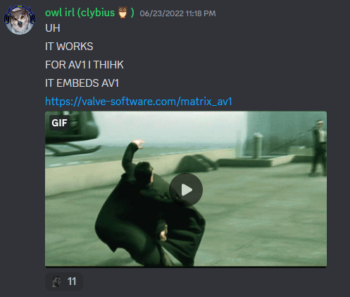
Clybius confirmed that this could be patched if discovered. He cites having had the idea from the Dwayne Johnson example above, but forgetting about it for a couple of months. So, it seems this entire concept stemmed from a silly rickroll.

### The Experiments & Interactive Site
After the discovery of AV1 embedding, experimentation brought about the discovery that *any* video codec will work as long as the user can decode/play the codec and the container/extension is an MP4, MOV, or WebM. These are all traditionally web-compatible containers. If you're interested in learning about containers, please see the [Containers](/start-here/terminology/#container) section on the [Terminology](/start-here/terminology/) page.
This applies to HEVC, ProRes, [xHE-AAC](/codecs/audio/aac/#xhe-aac), and other bizarre codecs that are rarely seen on the Web.
While experimentating, Clybius converted one their idle domains `stolen.shoes` into an interactive embedder that provided a textbox for a video URL, a thumbnail URL, a width value, & a height value for the desired video. This would be the first website for Discord embedding.
### Virality
It's not long before people outside of the AV1 Community discovered `stolen.shoes`, and its popularity increased rapidly. Its use usually involved the illicit distribution of full-length, unauthorized copies of movies; this sometimes happened very shortly after some movies were released. There were a couple notable instances of this happenening that caused quite the stir online each time.
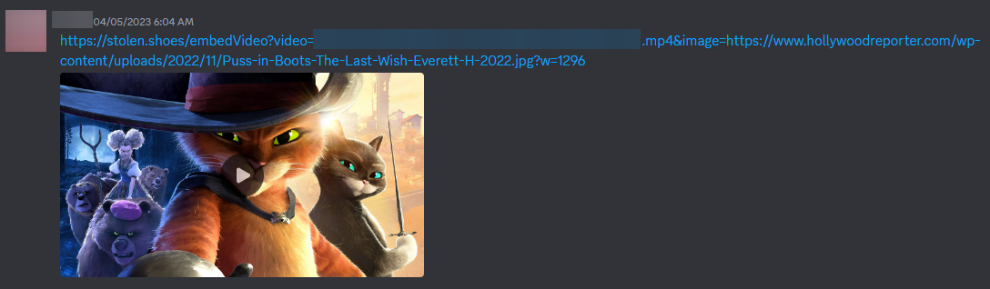
- The first instance featured the DreamWorks sequel of "Puss in Boots (2011)", "Puss in Boots: The Last Wish (2022)". A 1080p video sourced from a streaming site was the first wake up call that attracted attention to the existence of these embed sites. This example used `stolen.shoes`.
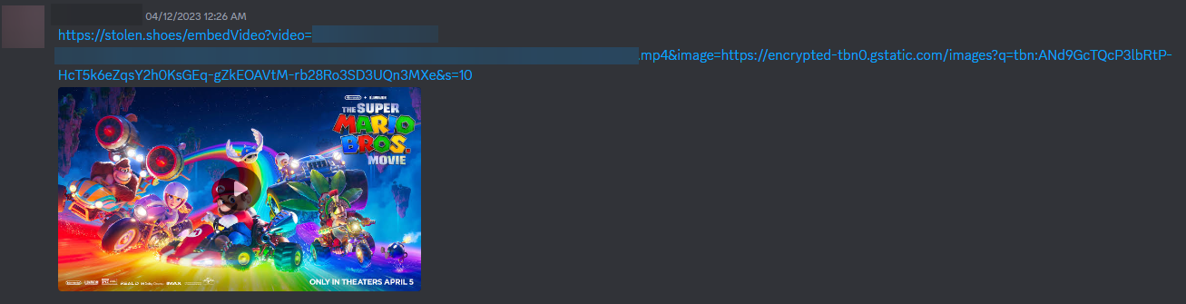
- The second instance was when highly-anticipated animated film "The Super Mario Bros. Movie (2023)" produced by Illumination, Universal Studios, and Nintendo was spread around Discord. It was first spotted as a Cam (A camera recording by someone in theaters), then as it went out on streaming services a different link appeared but spread faster and with upgraded 1080p quality. Both used `stolen.shoes` as the embed site.
- The third instance is very recent as of the day this was posted. A streaming-service sourced "Five Nights at Freddy's (2023)" was spread around since the movie released both in theaters and streaming service (Peacock) day one, and it gained steam extremely fast as most people had not seen it yet. Currently, this illegal novelty is gaining [hundreds of upvotes within the r/discordapp subreddit](https://www.reddit.com/r/discordapp/comments/17hx45y/is_discordnfp_an_ip_grabber/). The copy seems to be a compressed 720p encode. This example used `discord.nfp.is`.
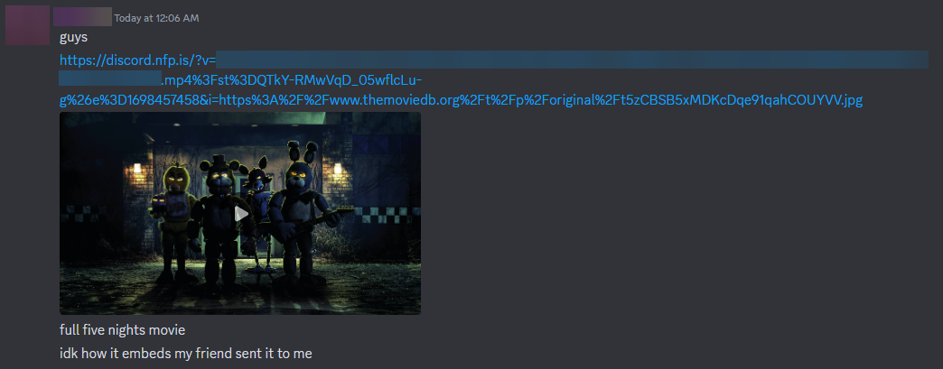
Note the ones listed here are the ones that I saw become extremely popular. There may be lesser known links that have been spread around privately or just did not cause enough noise for me to notice. Some less popular examples I've noticed, featuring more illicit copyrighted content distribution:
- Top Gun Maverick (2022)
- The SpongeBob trilogy (2005/2015/2020)
- Spider-Man: Across the Spider-Verse (2023)
## Closing
The ability to embed unusually large videos on Discord has enabled both positive and negative use cases. On the one hand, it allows high-quality content to be shared easily among friends. However, it has also facilitated mass copyright infringement by empowering virtually anyone with a Discord accound to freely spread pirated movies.
While this is fascinating from a technical perspective, embedding techniques like these tread a fine ethical line. As with anything, it is important to be mindful of how our actions affect others, and I should remind everyone that content creators deserve to be compensated for their work. As users, we should support them by accessing their content via legitimate platforms.
It is hard to say how long this exploit will continue to be usable. Instead of enabling piracy, which may cause Discord to be more likely to patch this exploit if they see it as a serious threat, let's instead use these capabilities responsibly to share our own creations, gaming highlights, and other media which we can share legally. Given some thoughtfulness, perhaps we can find a fair balance between respecting copyright law and appeasing Discord's sensibilities while allowing some creative flexibility on the platform.
Thank you for reading this blog post, I hope you learned something!
---
# Reducing Image Load Online
Canonical URL: https://encode.wiki/articles/site-optimization/
Collection: articles
Status: needs-review
License: CC BY-SA 4.0
Checksum: b673a1da8857b20dd1b2fafa9a1ab9083fa63b82a62d123597c2ce8f40d5f482
A big part of understanding any multimedia codec technology is knowing the application for such technology. For images, a big use case is web delivery. Compared to other multimedia, images are incredibly popular on the Web & knowing how to serve them properly can be a massive boon to your website's traffic as well as less of a headache for users on slower connections or who are under bandwidth constraints. The most disappointing part is that images are often poorly done on the web; all too frequently will you run into a site serving massive photographic PNGs for no reason, or photography sites serving photographs fresh out of the editing software with no thought put into their final delivery. A little effort, patience, & knowledge will go a long way toward improving the user experience for individuals using your site, & this article will illustrate some of the basics.
> **Caution — These instructions are for *photographic* images; other kinds of images, like non-photographic, artwork, pixel art, etc. should likely be handled differently..**
>
>
> **Danger — Many images won't load properly unless your browser supports JXL, AVIF, & proper ICCv2 color management. This is for demonstration purposes only & shouldn't represent an actual common website experience. If you're curious anyway, the following browsers can display the contents of this page perfectly:.**
>
> - [Thorium](https://thorium.rocks/) | *Linux, [macOS](https://github.com/Alex313031/Thorium-Special/releases), [Windows](https://github.com/Alex313031/thorium/releases/), [Android](https://github.com/Alex313031/Thorium-Special/releases)*
> - [Waterfox](https://www.waterfox.net/) | *[Linux](https://flathub.org/apps/net.waterfox.waterfox), [macOS](https://www.waterfox.net/download/), [Windows](https://www.waterfox.net/download/)*
> - [Mercury](https://thorium.rocks/mercury) | *[Linux](https://github.com/Alex313031/Mercury/releases), [Windows](https://github.com/Alex313031/Mercury/releases)*
## Fire & Forget
First, we'll illustrate what *not* to do, which is fortunately not incredibly difficult to avoid. Taking an image straight out of your editing software at a massive size will often bloat the size & resolution to something that isn't generally usable for a website regardless of the codec you're using & its quality per bit. It can be argued there are specific use cases that demand incredible resolution & fidelity coexist on the Web, but we won't be covering those here. Here's an example of a bloated image:
*exported straight from Darktable at JPEG q90, with no scaling*
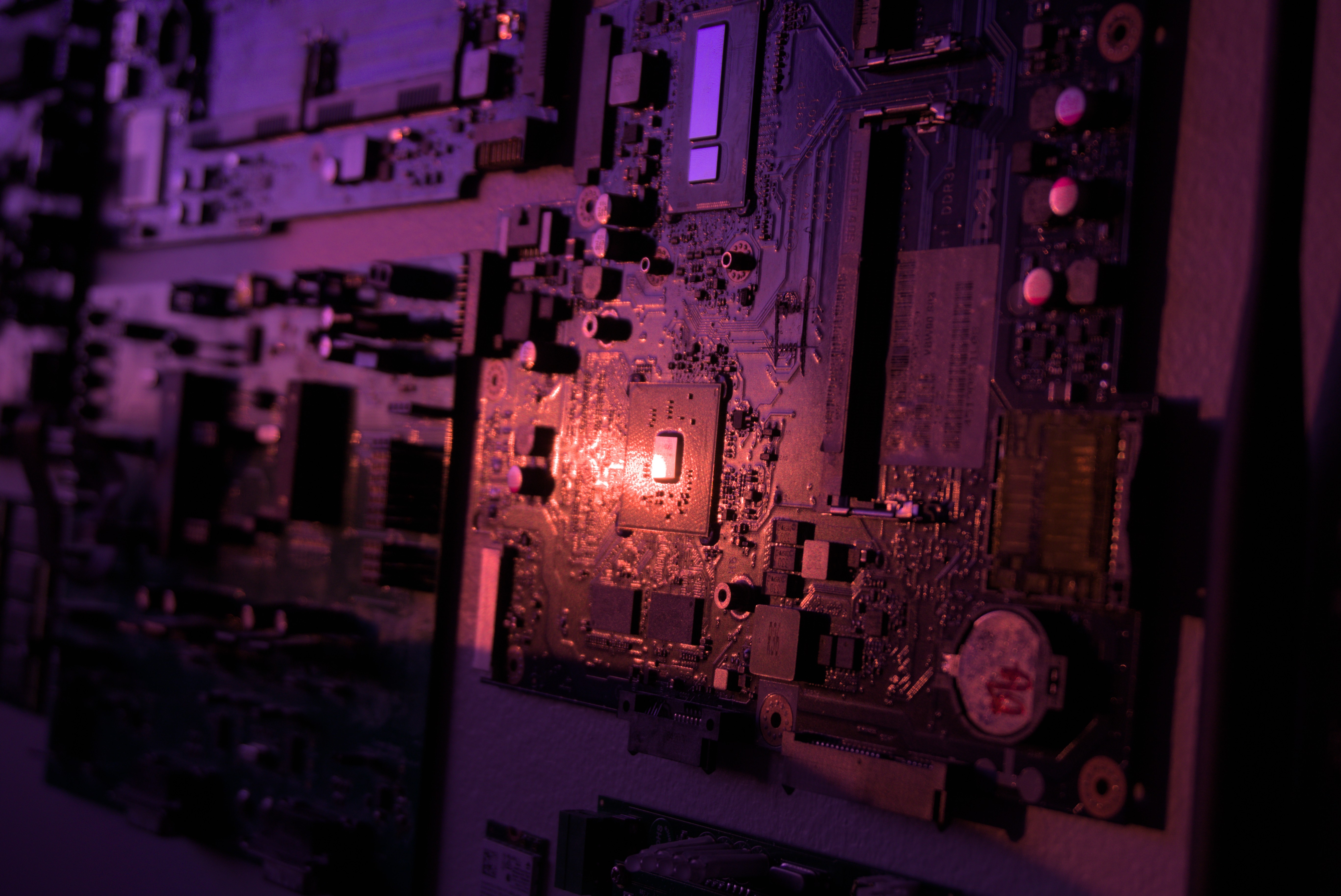
**2.2 MB**
## Massive Improvement
The easiest way to have a large improvement without doing much work is to simply resize the image before serving it. Even if you exported a lossy JPEG, resizing should remove a lot of artifacts. The way to perceive a worst-case for an image's size on a site is to inspect the image element's width & height, which should give us an estimate of how large we should make our image. Any larger than this value is unreasonable since we're overfilling the element's size for no reason & the image is being scaled down anyway.
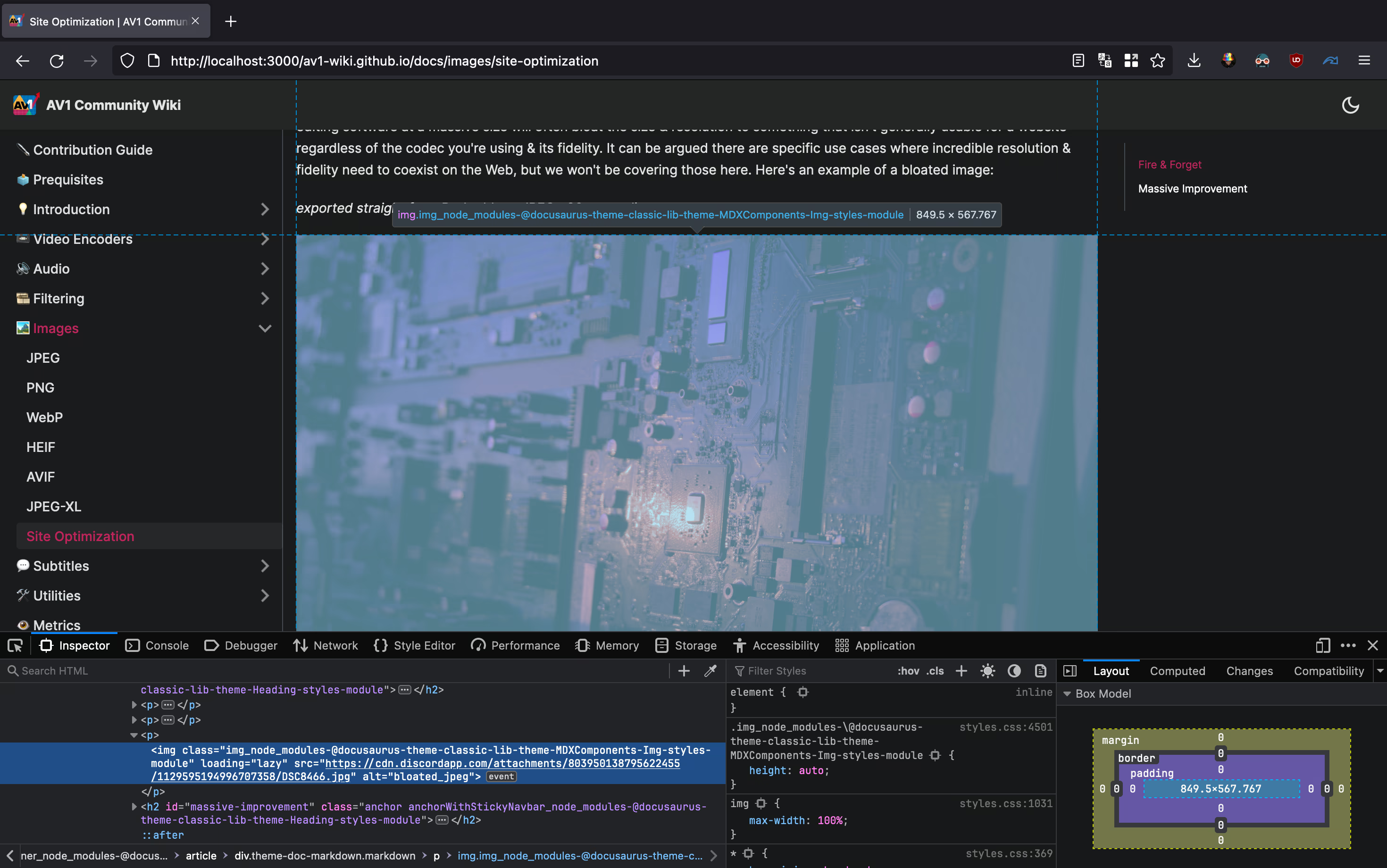
*Inspect Element in Firefox. The Mac used to take this screenshot has a relatively high display resolution of 2560x1664. Because Macs scale things differently, we're probably going to want to double the horizontal resolution here.*
The width is the most important value here, so our new image is going to be exported with a width of 1699 pixels. This new image, encoded at JPEG q90 with `cjpegli`, looks like this:
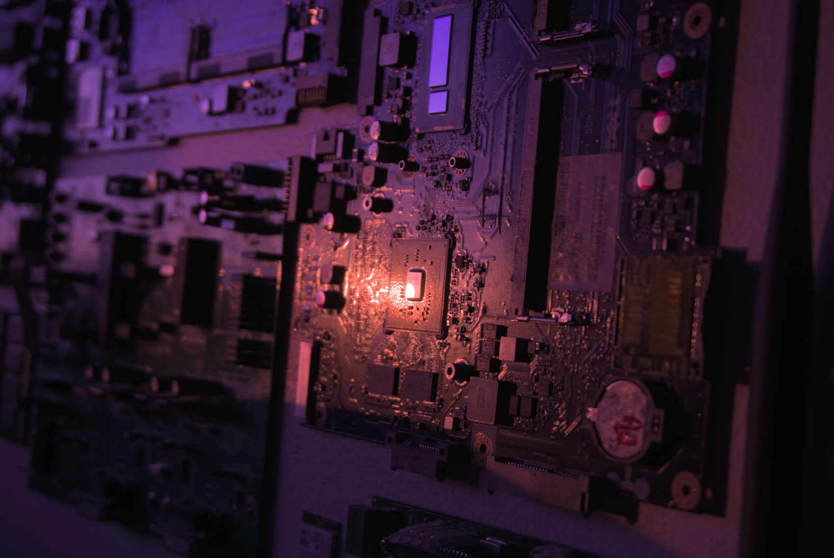
Obviously, there's lost fidelity compared to the original, but considering this is *so much smaller*, it is worth the trade-off for many. It is also worth noting we are using an improved jpeg encoder in the form of `cjpegli`, although that is secondary to the resize. If it doesn't look as good as you want it to, you can always scale the resolution up a bit, though currently, it looks plenty passable for its size.
2.2 MB -> **233 kB**
> **Chart — Page-weight reduction in the article example.** Resizing and re-encoding reduces the example image to roughly one tenth of its original transfer size. Data: Original: 2200 kB; Optimized: 233 kB.
### Lazy Loading
A bonus tip is to add the `loading="lazy"` attribute to your picture tag to allow the image to load only when scrolled to by a user. This doesn't save bandwidth, but it improves the user experience by loading images further down the page only when necessary. An example may look like this:
```html
```
## New Codecs
If you desire further improvement, it may be time to consider using a newer codec like [AVIF](/codecs/images/avif/) or [JPEG-XL](/codecs/images/jxl/). These options will compress far more effectively than JPEG, with the only trade-off being browser support. We're not going to consider [WebP](/docs/images/WebP) or [HEIC](/docs/images/HEIC), since WebP is not competitive enough with JPEG for photographic imagery (often being worse) & HEIC has been superseded by AVIF - which sees greater support anyhow - & is not royalty free, effectively preventing widespread Web adoption forever. Again, we're just considering *lossy* compression for *photographic* images; it is a different story with WebP elsewhere, as it performs well on non-photographic content & is almost always better than PNG for 8-bit lossless compression. So, we are left with JXL & AVIF for now.
### Fallbacks
AVIF sees widespread support, but JPEG-XL isn't quite there yet with Web support as Google continues to push AVIF (it is debatable if it ever will be outside the Apple ecosystem). Even with AVIF, adoption isn't remotely close to JPEG, so it is worth providing a fallback. This can look like the following example:
```html
```
Here is a JXL falling back to an AVIF falling back to a WebP falling back to a JPEG. Pretty intense to have this many fallbacks unless you're really after the ultimate compression ratio, but it is certainly an option. AVIF & JPEG alone will probably be enough for most.
### Compression Efficacy
Let's look at how our image examples compare to the original with our new codec selection. We'll be aiming for high visual fidelity, so around the same quality as our initial JPEG encoded with `cjpegli` (which scores ~`83.01` with the [SSIMULACRA2](/docs/metrics/SSIMULACRA2) visual fidelity metric).

**137.0 kB** *JPEG-XL image, encoded with `cjxl lossless.png out.jxl -d 1.49 -e 9`. Score: ~`83.04`* *3.06s user time*

**124.8 kB** *AVIF image, encoded with `avifenc -c aom -s 4 -j 8 -d 10 -y 444 --min 1 --max 63 -a end-usage=q -a cq-level=16 -a tune=ssim lossless.png out.avif`. Score: ~`83.03`* *7.54s user time*
JXL also supports lossless transcoding of JPEG images. This means every pixel is identical, the image just has a smaller filesize than the original JPEG; if you can use JXL, you can transcode existing JPEGs losslessly on your site & save some bandwidth that way. The JPEG transcode below gives a higher SSIMULACRA2 score than the original for some reason, but I'll chalk that up to a decoding inconsistency between how the `ssimulacra2` program decodes JPEG & JXL. Either way, the scores are fairly close.

**189.4 kB** *JPEG-XL image from JPEG, encoded with `cjxl input.jpg input-recomp.jxl -d 0.0 -e 9 --brotli_effort=11`. Score: ~`84.92` (???)* *0.67s user time*
The final trick we can use, while not a new codec at all, still increases quality per bit. Encoding an XYB JPEG with `cjpegli` encodes with the perceptual XYB colorspace using an ICC profile to modify the original JPEG colors, avoiding JPEG's normal YCbCr which isn't perceptually optimized for the human visual system. Using XYB, we can afford identical quality with less bitrate than normal JPEG. This has universal compatibility, but not every application understands how to handle the XYB color profile (although color-managed modern browsers should be fine).

**208.3 kB** *XYB JPEG, encoded with `cjpegli lossless.png out.jpg --xyb -d 1.155`. Score: ~`83.04`* *0.10s user time*
In this particular instance, AVIF seems to be the overall winner. This isn't always the case due to JXL's superiority at higher fidelity & with more detailed images, but according to SSIMULACRA2, AVIF has the best quality per bit with this image. You can use your own eyes to further clarify your choice, though. It is worth mentioning that as these were encoded from a 16-bit source PNG, the JXL image is the only one that maintains the full original bit depth, & AVIF isn't fast to encode.
## Responsive Images
Displaying an image that is too large for a viewport is a waste of bandwidth, & displaying an image that's too small for the viewport leaves fidelity to be desired. Luckily, we have the [Responsive Image Linter](https://ausi.github.io/respimagelint/) that can help us figure out which image sizes we should be using.

In our fire & forget example, we see that we are serving an image that is far too large. We already know that, but now we can see that given various viewport sizes we could be serving images that have respective widths of 270px, 958px, 1350px, 1660px, & 1916px to optimize for delivery to a variety of different devices. Here's how we'd write that in HTML:
```html
```
It is worth noting that this example above & the example below aren't perfect implementations of a responsive image given the conditions of this site, but the general concept still applies. Some things to note:
- `srcset` = the images available to your browser to serve, & their respective widths
- `sizes` = the conditions given to the browser explaining under what conditions should it serve which image
- `(min-width: XXXpx) YYYpx` = Given the viewport is at least XXX wide, serve an image of YYY horizontal resolution. The browser will pick an image from srcset that is CSS pixels \* display scaling.
- `calc(100vw - 24px)` = Usually preceded by a (min-width) condition. Specifies a value the browser should calculate on its own to pick the closest option from the srcset. Let's say we have `(min-width: 997px) calc(75vw - 257px)`. This means given the viewport is at least 997px wide, calculate 0.75 \* the current viewport resolution - 257 to find the closest image in the srcset to fit the number of pixel specified.
That's all! Massive thanks to Auto-Rez Media Technologies for the inspiration behind this article & explicit permission to use their [Reduce Your Page's Image Load](https://autocompressor.net/blog/reduce-image-load) blog post when writing this entry. I have [confirmed](https://autumn.revolt.chat/attachments/GtFGuwNfeRdcwUN0MWzhDCAiiadWOk88XXC3pQv6RI) with their leadership that this wiki entry can be safely licensed under CC BY-SA 4.0.
---
# Encoding Animation with SVT-AV1: A Deep Dive
Canonical URL: https://encode.wiki/articles/svt-av1-deep-dive/
Collection: articles
Status: needs-review
License: CC BY-SA 4.0
Checksum: 8ec837249aa678752f367a55d42085da4fa2acacca0740072e1146dd1489afa5
# Introduction
This blog post is based on a series of visual quality benchmarks with SSIMULACRA2 and speed benchmarks of SVT-AV1 1.8.0 on a corpus of animated clips.
The resources available will range from ***graphs*** to ~~**image comparisons**~~ (WIP). The ***former*** has the advantage of being easily understandable, showcasing pure efficiency comparisons between encoder parameters using metrics as the reference, while the **latter** are image samples from the encoded files during the tests that enable you to check quality for yourself and add another layer of subjective interpretation to these comparisons.
The testing methodology involves using relatively short video samples from a wide range of modern anime genre, which have been either losslessly encoded with `x264 --qp 0` for ease of use or losslessly cut from their source. These lossless files are then pipped into SvtAv1EncApp *directly*, meaning we are measuring the performance of a single encoder instance and not leveraging chunked encoding like any actual final AV1 encoding pipeline should. Once an encode is done, SSIMULACRA2 scores are calculated using the [Zig implementation](https://github.com/dnjulek/vapoursynth-ssimulacra2) and lots of useful data are aggregated to make the graphs for this benchmark, including encoding time, encode size (bitrate), and SSIMULACRA2 scores. Bits per pixel scores (BPP) are calculated so that the `Metric / BPP` graphs may represent the closest we have to real efficiency.
The clips used in this test were acquired legally. The Codec Wiki and its contributors do not endorse media piracy.
SvtAv1EncApp was compiled directly from the [v1.8.0 source code](https://gitlab.com/AOMediaCodec/SVT-AV1/-/releases/v1.8.0) using the provided `Build/linux/build.sh` script, Clang 16.0.6, and Profile-Guided Optimization (PGO). The testing machine is comprised of an i7 8750H running at 35W with 16GB of 2666MHz DDR4 RAM in Arch Linux with kernel 6.6.6 and the performance governor enabled. All encodes have been made in the same session without rebooting.
This testing was conducted within the [AV1 Weeb Edition](https://discord.gg/83dRFDFDp7) Discord server, which is focused on encoding animated content in AV1.
## Samples
The samples are as follows:
- 11s `Blame!` clip which sports 3DCG action with lots of grain, effects and high-contrast elements. Most complex source of this set.
- 13s `Blue Lock` clip which sports rapid camera movements and rotations + high-contrast elements.
- 15s `Fate/Grand Order: Babylonia` relatively slow-paced clip with lots of effects still. Easiest source of this set but easy sources still give interesting data.
- 22s `Jigokuraku (Hell's Paradise)` flashback clip with huge static grain in a very dark scenery and some action.
- 14s `Kaguya-sama` opening sequence with lots of effects and fast change of scenery.
The resolution of every clip is 1080p, except for the first one which is 1920x804.
> **All clips have been encoded in a wide quality range, from `--crf 8` to `--crf 43`.**
Without further ado, let's start with the first comparisons!
## Presets comparisons (-1 -> 13)
**In the following graphs, you may find comparisons between all SVT-AV1 presets, ranging from the slowest `--preset -1` to the fastest `--preset 13`.**
*Please remember that these two extreme presets are meant for development purposes and as such should not be used in normal encoding conditions. You will soon understand why.*
`--preset X` is the only parameter used here, in conjunction with the CRF values. That means everything else is default. The defaults worth mentioning are:
- `--tune 1`: tune PSNR
- `--aq-mode 2`: variance deltaq
- `--enable-qm 0`: quantisation matrices disabled
- `--irefresh-type 2`: closed GOP
- `--enable-tf 1`: temporal filtering enabled
And more, like CDEF and restoration enabled, overlays and film-grain disabled...
- First of all, here are the efficiency graphs:
> **Interactive comparison:** [Open the complete media manifest](/media/articles/svt-av1-deep-dive.json).
This could be too much information.
- Now the same graphs but focusing on the "high quality" range (CRF8 -> 23):
> **Interactive comparison:** [Open the complete media manifest](/media/articles/svt-av1-deep-dive.json).
- Same again but without presets 9 to 13 for better clarity:
> **Interactive comparison:** [Open the complete media manifest](/media/articles/svt-av1-deep-dive.json).
- Now for the "low quality" range (CRF28 -> 43):
> **Interactive comparison:** [Open the complete media manifest](/media/articles/svt-av1-deep-dive.json).
- Same but without presets 9 to 13 for better clarity:
> **Interactive comparison:** [Open the complete media manifest](/media/articles/svt-av1-deep-dive.json).
- **Let's now see speed comparisons between all presets:**

As we can see, preset -1 is so abysmally slow it makes the graph unusable
(BTW, notice the `1e6` in the lower right corner, it is obviously not encoding at 1 to 4 ms, but at 1 000 000 to 4 000 000 ms)
- Here is what it looks like with a logarithmic scale:
> **Interactive comparison:** [Open the complete media manifest](/media/articles/svt-av1-deep-dive.json).
- **Now the speed graphs but with SSIMU2 on the y-axis instead of BPP: (logarithmic scale)**
> **Interactive comparison:** [Open the complete media manifest](/media/articles/svt-av1-deep-dive.json).
- Here are speeds graphs for preset 1 to 6 with a linear scale:
> **Interactive comparison:** [Open the complete media manifest](/media/articles/svt-av1-deep-dive.json).
One interpretation we can have is that **presets 2 to 4** have actually pretty close scores (pretty much the same at HQ, 2 points at max in the low quality range) but **preset 2** is **2x slower than preset 4**. The quality gap between **preset 2** and **preset 1** is even narrower but the speed penalty is also ~2x.
That makes it hard to recommend **preset 1**, while **preset 3** is in a strange middle ground between **2** and **4** where it makes little sense to choose it over those two: it's better to choose **preset 2** for the higher efficiency at 1.5x slower speeds, or **preset 4** for the 1.33 to 1.5x higher speeds. At least the option exists.
A similar observation can be made between **preset 5** and **6**. They can be so close in scores in many samples (especially at HQ) while also being close in speeds that **preset 5** becomes rather obsolete most of the time.
### TLDR
**Clear quality gains can be observed as we decrease presets, until the very last one, however the effectiveness of dropping presets becomes less and less impressive the higher in quality you go.**
- For instance, in worst-case scenario, we observe that (for the CRF23 to CRF8 range), __**preset 4**__ only loses at maximum **2** SSIMU2 **points** compared to __**preset -1**__ while being 50-60x faster. Though to be fair, the speed loss from __**preset 4**__ to __**preset 0**__ is "only" 5-10x for a maximum SSIMU2 difference close to **1.5 point**.
- From CRF43 to CRF28, the difference between __**preset 4**__ and __**preset -1**__ can be as much as **5** SSIMU2 **points**, so lower presets become more attractive.
## Tunes comparisons
**In the following graphs, you may find comparisons between SVT-AV1 tunes, from the default `--tune 1` (PSNR) to the other two tunes: `--tune 0` (VQ) and `--tune 2` (SSIM).**
Except for the tunes, `--preset 4` is set due to its good balance of quality and speed, in conjunction with the CRF values. That means everything else is default. The defaults have been mentioned earlier above.
- **Let's compare the efficiency of every tunes:**
> **Interactive comparison:** [Open the complete media manifest](/media/articles/svt-av1-deep-dive.json).
- Now let's focus on the "high quality" range (CRF8 -> 23):
> **Interactive comparison:** [Open the complete media manifest](/media/articles/svt-av1-deep-dive.json).
- And the "low quality" range (CRF28 -> 43):
> **Interactive comparison:** [Open the complete media manifest](/media/articles/svt-av1-deep-dive.json).
- And here is the speed difference:
> **Interactive comparison:** [Open the complete media manifest](/media/articles/svt-av1-deep-dive.json).
- Graphs comparing the tunes individually between each others will be made available soon.
- The image comparisons will make the conclusion quite more nuanced, stay tuned (heheh) for that.
### TLDR
**SSIMU2 favors __tune 1 and 2__ above __tune 0__. At high quality, __tune 1 and 2__ are matched, while at low quality __tune 2__ takes the edge. __Tune 0__ is sometimes a match for the other two on certain clips and other times fare pretty badly.**
**For some reason, __tune 0__ is quite a bit faster now, compared to 1 and 2 which are basically the same.**
Keep in mind that I have observed multiple times in the past that __tune 0__ kept more fine detail and was sharper than the other tunes, at the expense of potential artifacting, like ringing and distortion. It may very well explain why the metric doesn't like its results. The image comparisons may give a different interpretation than what we concluded here, please stay *tuned* for these subjective comparisons.
## Parameters comparisons
**In the following graphs, you may find comparisons between many SVT-AV1 parameters.**
*Additional graphs focusing on the high and low qualities will be made available later down the line*
`--preset 4` is used here due to its good balance of quality and speed, in conjunction with the CRF values. That means everything else is default. The defaults have been mentioned earlier above.
### `--tile-rows 1 --tile-columns 1` vs default `--tile-rows 0 --tile-columns 0`
- Efficiency graphs:
> **Interactive comparison:** [Open the complete media manifest](/media/articles/svt-av1-deep-dive.json).
- Speed graphs:
> **Interactive comparison:** [Open the complete media manifest](/media/articles/svt-av1-deep-dive.json).
> __tiles__ here are both slightly harmful and slower.
### `--aq-mode 0` vs default `--aq-mode 2`
- Efficiency graphs:
> **Interactive comparison:** [Open the complete media manifest](/media/articles/svt-av1-deep-dive.json).
- Speed graphs:
> **Interactive comparison:** [Open the complete media manifest](/media/articles/svt-av1-deep-dive.json).
> Except for the Jigokuraku clip, __aq-mode 0__ is harmful in the eyes of SSIMU2, while being slower at low CRF levels, and sometimes a match or faster at high CRF levels.
### `--aq-mode 1` vs default `--aq-mode 2`
- Efficiency graphs:
> **Interactive comparison:** [Open the complete media manifest](/media/articles/svt-av1-deep-dive.json).
- Speed graphs:
> **Interactive comparison:** [Open the complete media manifest](/media/articles/svt-av1-deep-dive.json).
> __aq-mode 1__ fares closer to __aq-mode 2__ than __aq-mode 0__ did, both in quality and speed, but is still overall inferior according to SSIMU2
### `--enable-cdef 0` vs default `--enable-cdef 1`
- Efficiency graphs:
> **Interactive comparison:** [Open the complete media manifest](/media/articles/svt-av1-deep-dive.json).
- Speed graphs:
> **Interactive comparison:** [Open the complete media manifest](/media/articles/svt-av1-deep-dive.json).
> According to SSIMU2, disabling CDEF barely impact efficiency. But as its a pretty demanding tool, there's a slight speed benefit of having it disabled too. I advise you to take these results with a grain of salt until the image comparisons, because in anime particularly, CDEF *can* be beneficial for the line-art.
### `--enable-dg 0` vs default `--enable-dg 1`
- Efficiency graphs:
> **Interactive comparison:** [Open the complete media manifest](/media/articles/svt-av1-deep-dive.json).
- Speed graphs:
> **Interactive comparison:** [Open the complete media manifest](/media/articles/svt-av1-deep-dive.json).
> __Dynamic GoP control__ yields bit-perfect results in all clips except for Blue Lock and Jigokuraku. There is no speed benefit to disabling it except in clips where it is in use. Let's not jump to conclusions too easily, the image comparisons will tell if it's "safe" to keep the setting disabled at all times or not.
### `--enable-dlf 0` vs default `--enable-dlf 1`
- Efficiency graphs:
> **Interactive comparison:** [Open the complete media manifest](/media/articles/svt-av1-deep-dive.json).
- Speed graphs:
> **Interactive comparison:** [Open the complete media manifest](/media/articles/svt-av1-deep-dive.json).
> __Deblocking loop filter__ can be slightly beneficial in some scenarios. In reverse, it is never harmful, so it is recommended to keep it default.
### `--fast-decode 1` vs default `--fast-decode 0`
- Efficiency graphs:
> **Interactive comparison:** [Open the complete media manifest](/media/articles/svt-av1-deep-dive.json).
- Speed graphs:
> **Interactive comparison:** [Open the complete media manifest](/media/articles/svt-av1-deep-dive.json).
> __fast-decode 1__ is pretty harmful in the Fate clip and slightly harmful in the rest. There is a speed benefit of enabling it though.
### `--irefresh-type 1` vs default `--irefresh-type 2`
- Efficiency graphs:
> **Interactive comparison:** [Open the complete media manifest](/media/articles/svt-av1-deep-dive.json).
- Speed graphs:
> **Interactive comparison:** [Open the complete media manifest](/media/articles/svt-av1-deep-dive.json).
> Finally something interesting to analyse!
- __irefresh-type 1__ is either a match or beneficial compared to __irefresh-type 2__ at high CRF levels.
- __irefresh-type 1__ either wins or lose to __irefresh-type 2__ at low CRF levels depending on the clip. As such, it is NOT recommended to blindly set __irefresh-type__ to __1__ at "high quality" as it might be harmful depending on the content.
- __irefresh-type 1__ is always slower compared to __irefresh-type 2__, so I might argue it is more safe to leave __irefresh-type__ default at "high quality" than not.
- According to the content type of those clips, it appears that __irefresh-type 1__ may benefit *extremely grainy* content while default __irefresh-type 2__ is better suited for *cleanish* content. This needs to be confirmed with *moar* testing though.
### `--lookahead 0` vs default `--lookahead -1` (auto)
- Efficiency graphs:
> **Interactive comparison:** [Open the complete media manifest](/media/articles/svt-av1-deep-dive.json).
- Speed graphs:
> **Interactive comparison:** [Open the complete media manifest](/media/articles/svt-av1-deep-dive.json).
### `--lookahead 60` vs default `--lookahead -1` (auto)
- Efficiency graphs:
> **Interactive comparison:** [Open the complete media manifest](/media/articles/svt-av1-deep-dive.json).
- Speed graphs:
> **Interactive comparison:** [Open the complete media manifest](/media/articles/svt-av1-deep-dive.json).
### `--lookahead 120` (max) vs default `--lookahead -1` (auto)
- Efficiency graphs:
> **Interactive comparison:** [Open the complete media manifest](/media/articles/svt-av1-deep-dive.json).
- Speed graphs:
> **Interactive comparison:** [Open the complete media manifest](/media/articles/svt-av1-deep-dive.json).
> __lookahead__ seems to behave strangely when set...
- __lookahead 0__ shifts quality around a lot and it is difficult to draw conclusions but there's a clear speed drawback of disabling lookahead.
- __lookahead 60__ is perfectly bit-perfect to every clips EXCEPT for some damn reason in Jigokuraku at CRF23
- __lookahead 120__ is somehow also bit-perfect, but this time in every clips and every CRF levels. Both 60 and 120 don't see much speed differences.
> Soooo.... this behavior is so odd I don't advise to set any lookahead value. Let the encoder decide.
### `--enable-overlays 1` vs default `--enable-overlays 0`
- Efficiency graphs:
> **Interactive comparison:** [Open the complete media manifest](/media/articles/svt-av1-deep-dive.json).
- Speed graphs:
> **Interactive comparison:** [Open the complete media manifest](/media/articles/svt-av1-deep-dive.json).
> __overlays__ do not seem to either improve efficiency or performance.
### `--enable-qm 1` vs default `--enable-qm 0`
- Efficiency graphs:
> **Interactive comparison:** [Open the complete media manifest](/media/articles/svt-av1-deep-dive.json).
- Speed graphs:
> **Interactive comparison:** [Open the complete media manifest](/media/articles/svt-av1-deep-dive.json).
> Enabling __quantization matrices__ alone increase efficiency at "high quality" with no real speed impact.
### `--enable-qm 1 --qm-min 0` vs `--enable-qm 1`
- Efficiency graphs:
> **Interactive comparison:** [Open the complete media manifest](/media/articles/svt-av1-deep-dive.json).
- Speed graphs:
> **Interactive comparison:** [Open the complete media manifest](/media/articles/svt-av1-deep-dive.json).
> Setting __qm-min__ to __0__ on top of enabling __quantization matrices__ can be beneficial in some clips at no added compute time.
I will re-tests many QMs ranges in the future, but I doubt it changed much from v1.7.0 where 0 was the most appropriate choice for most content.
### `--enable-restoration 0` vs default `--enable-restoration 1`
- Efficiency graphs:
> **Interactive comparison:** [Open the complete media manifest](/media/articles/svt-av1-deep-dive.json).
- Speed graphs:
> **Interactive comparison:** [Open the complete media manifest](/media/articles/svt-av1-deep-dive.json).
> Even though the efficiencies are very similar, nothing is bit-perfect here. So according to SSIMU2, the __loop restoration filter__ isn't necessarily useful. However, just like CDEF, it's a pretty demanding tool, so disabling it yields some performance improvements. Let's take these with a grain of salt until the image comparisons.
### `--scm 0` vs default `--scm 2` (content adaptive)
In all the clips, the results are bit-perfect and there is no notable performance difference.
### `--scm 1` vs default `--scm 2` (content adaptive)
- Efficiency graphs:
> **Interactive comparison:** [Open the complete media manifest](/media/articles/svt-av1-deep-dive.json).
- Speed graphs:
> **Interactive comparison:** [Open the complete media manifest](/media/articles/svt-av1-deep-dive.json).
> Interestingly enough, __screen content tools__ seem to improve efficiency according to SSIMU2, at the cost of a huge performance regression. After the image comparisons are published, I will conduct additional testing on this.
### `--enable-tf 0` vs default `--enable-tf 1`
- Efficiency graphs:
> **Interactive comparison:** [Open the complete media manifest](/media/articles/svt-av1-deep-dive.json).
- Speed graphs:
> **Interactive comparison:** [Open the complete media manifest](/media/articles/svt-av1-deep-dive.json).
> Disabled __temporal filtering__ *can* sometimes improve efficiency slightly at "high quality", however it is very much clip dependent. It also improves performance slightly. The image comparisons will give another perspective to these results.
### `--enable-tpl-la 0` vs default `--enable-tpl-la 1`
In all the clips, the results are bit-perfect and there is no notable performance difference.
### `superres`:
Kinda lazy to make, share and comment so much graphs for something that can be told in two lines...
All superres variants are freaking useless as they:
- do not improve efficiency
- decrease encoding speeds
- decrease decoding speeds when either bitrate or quality normalized.
### __Early TLDR on parameters results:__
***For a previous test with SVT-AV1 1.7.0 I did all parameters tests with `--preset 6 --tune 2`, now I did them with `--preset 4 --tune 1`. Mostly everything tested on v1.7.0 still stands today, but now we have more valuable data. Images comparisons are still needed to give more context to some results, so the conclusion presented here remains early as they are 100% based on SSIMU2 results and will require more analysis down the line.***
**Here is a quick run down of how each parameter affect encoding:**
- `--tile-rows --tile-columns` should never be used (except for decreasing decode complexity)
- `--aq-mode 2` is the most efficient / fastest
- `--enable-cdef 0` *might* improve performance at almost no efficiency loss *(needs more thorough testing)*
- `--enable-dg` and `--enable-dlf` barely do anything
- `--fast-decode 1` decreases efficiency, improves encoding times, and the decoding gains still need to be determined.
- `--irefresh-type` should be kept default at high CRF values and for cleanish content at low CRF values, but can be set to 1 at low CRF values for extremely grainy content
- `--lookahead` should be kept default
- `--enable-overlays 1` does not improve efficiency, slight speed regression as well
- `--enable-qm 1 --qm-min 0` should be set for increased efficiency especially at low CRF values at no perf cost
- `--enable-restoration` barely does anything but disabling yields better performance *(needs visual confirmation)*
- `--scm 1` screen content tools can improve efficiency with a big performance trade-off *(needs more thorough testing)*
- `--enable-tf 0` is a mixed bag efficiency wise but improves performance
- `superres & resize` please don't.
## Conclusion
The extensive benchmarking reveals that obviously the slower presets provide better efficiency, with diminishing returns past preset 2. However, preset 4 provides a good balance of quality and speed for most use cases. Presets 6 and 8 are good options for the people that find 4 to be too slow for their liking.
The default settings tend to provide good results, but some tweaks like enabling quantization matrices can further optimize efficiency. Parameters like tile encoding and super resolution modes are not beneficial. Overall, SVT-AV1 continues to be a competitive option for encoding animation in AV1, with its speed being a notable strength.
Further testing with more content samples would help solidify these findings. The image comparisons will also provide additional subjective evaluation to complement the objective metrics used here, and we can discover the potential usefulness of Tune 0 that may betray what the metrics suggest. Overall, this comprehensive deep dive should give encoders a helpful starting point for choosing settings when encoding animation with the latest SVT-AV1 1.8.0. Thanks for reading!
{}
---
# Deep Dive into SVT-AV1's Evolution (Part 1): Presets Analysis from v2.0 to v3.0
Canonical URL: https://encode.wiki/articles/svt-av1-fourth-deep-dive-p1/
Collection: articles
Status: needs-review
License: CC BY-SA 4.0
Checksum: b5faa036017e5c781c2459c99f31f92b12ca39a11f752a8d69fe8a63a1b9349b
# Introduction
It's been almost a year since SVT-AV1 v2.0.0 dropped in March 2024, and we finally got v3.0.0 in late February of this year. Minor versions v3.0.1 and v3.0.2 came along afterward with some bug fixes and ARM SIMD improvements, but they didn't meaningfully alter encoding results.
So what's actually different between these versions? I've been wanting to run tests across all the major releases from v2.0.0 to v3.0.x to see how the speed vs quality trade-offs have evolved this past year. Using SSIMULACRA2, Butteraugli, XPSNR, and VMAF (plus some methodology tweaks I'll get into), I'll break down what each version brought to the table and in a second part, we'll also deep dive a few specific options that appeared in the encoder since my first blog post release so you can figure out what you may want to use for your projects. That includes variance boost, fast decode, temporal filtering strength and a few others...
## Feedback
Although the reception was warm, I got less feedback than usual this time around, but honestly, that hasn't prevented me from wanting more. And better! I'm keeping the stuff that seemed well-received: the diverse test clips, visual comparisons, and my ongoing attempt to stay as objective as possible.
In my last post's conclusion, I mentioned some frustrations: XPSNR was acting up, metrics were taking forever to calculate, and there was just too much data to make sense of. Good news is I've tackled all of these. I fixed the XPSNR issue (it expected mod-8 inputs), started using the new [Vship](https://codeberg.org/Line-fr/Vship) to speed up metrics calculation, and found a cleaner way to present all the data points at just two quality levels, like I used to do.
Also, it needs to be pointed out I've been way too optimistic about how often I can get these posts out. Especially when I revamp the methodology each time. I'm sorry about that, again. Though, my ambition may also be at fault: the size of this article got so out of hand I eventually decided to split it into two parts for convenience's sake.
## Methodology
You'll find both graphs and visual comparisons in this analysis. The graphs give you objective data on encoder efficiency across different settings, using various metrics. The image comparisons show the actual encoded samples so you can judge quality for yourself, adding that subjective element that numbers alone can't capture.
This time, I'm using a new tool called [*Metrics*](https://github.com/psy-ex/metrics) from the self-proclaimed Psychovisual Experts group, which provides scripts for measuring and comparing video codecs. I've heavily modified these scripts for my specific needs, but if you want to run your own tests locally, definitely check out the original *Metrics* toolkit!
---
Here's how the testing works: I use relatively short video samples covering a wide range of content types, all converted to uncompressed y4m format (if they weren't already!) for consistency. These lossless files go straight into *SvtAv1EncApp*, so we're measuring single-instance encoder performance here. Keep in mind that serious AV1 encoding pipelines should probably use chunked encoding (with a tool like [Av1an](https://github.com/rust-av/Av1an)), especially on higher core count systems.
Once encoding is done, we run multiple full-reference metrics comparing the encodes against the original source. Using several different metrics helps compensate for each one's weaknesses and gives a more complete picture of the actual visual differences between encodes. I try to stray away from the industry standard metrics which tend to have poor correlation to *Mean Opinion Scores* (MOS), and instead focus more on psychovisual metrics that better represent actual visual quality. I calculate *SSIMULACRA2* and *Butteraugli* scores using [Vship](https://codeberg.org/Line-fr/Vship), an accurate GPU-accelerated port of the Zig implementation I used before that's also much faster. *XPSNR* and *VMAF* scores come from their respective ffmpeg filters, but with a twist!
If you remember, last time I started making use of Harmonic Mean for SSIMU2 to better account for inconsistent scoring behaviors within a video. We'll be doing it again today.
This time sees the addition of the (in)famous VMAF metric, but in a radically different form than you've probably ever seen until now. Indeed, it is well known VMAF is rather [unreliable](https://arxiv.org/pdf/2107.04510), but with a few modifications to the scoring method, we can try to make it better. I'm computing scores across all three color planes (instead of just luma as VMAF isn't chroma aware), then weighting them with this formula: `((4.0 * vmaf_y) + vmaf_u + vmaf_v) / 6.0`. This approach is inspired by the now-unavailable better-vmaf mod. I also chose to use [VMAF's neg model](https://github.com/Netflix/vmaf/blob/master/resource/doc/models_v0.md#disabling-enhancement-gain-neg-mode) and to disable the motion component (`motion.motion_force_zero=true`) since it's notorious in our niche encoding communities for inflating scores during motion and producing nonsensical results (bad looking frames having near perfect scores...). I'll refer to this metric as W-VMAF in the rest of this post.
XPSNR gets similar treatment: motion component disabled ([by commenting out this line](https://github.com/FFmpeg/FFmpeg/blob/master/libavfilter/vf_xpsnr.c#L240)) and the same weighting formula: `((4.0 * xpsnr_mse_y) + xpsnr_mse_u + xpsnr_mse_v) / 6.0`. As you may glimpse from said formula, XPSNR's dB values are converted back to linear MSE, we then calculate the weighted average and convert back to dB. I'll refer to this metric as W-XPSNR in the rest of this post.
Butteraugli runs in stock configuration except for the intensity multiplier set to 203 nits instead of the currently default 80 (based on an [industry reference](https://www.itu.int/dms_pub/itu-r/opb/rep/R-REP-BT.2408-3-2019-PDF-E.pdf), used by MPV for instance).
I believe these modifications produce more meaningful results than stock metrics, but proving that is beyond this post's scope. You'll have to trust the methodology or test it yourself. All this data gets aggregated to create the benchmark graphs.
The "speed graphs" plot *Constant Rate Factor* (CRF) against encoding time to show speed efficiency at different quality targets. For compression efficiency, I plot metric scores against output file size. Since *Metrics* doesn't use *bits per pixel* (BPP) and I had received feedback a few blog posts back that this metric could be confusing, I decided to drop it this time around.
To achieve more accurate efficiency curves with fewer probes, it is more effective to prioritize probes in the higher-quality (lower CRF) range of the quality spectrum, since bitrate will increase quicker. I used the following formula, courtesy of better-vmaf's author, to determine ten CRF values from 10 to 50 to use for the testing: `crfs = [min_q + (max_q - min_q) * ((step / (q_steps - 1)) ** scaling_factor) for step in range(q_steps)]`, then equally split into *High Quality* and *Low Quality* graphs and visual comparisons.
How to read the graphs? For the compression efficiency graphs, higher and further left is better, except for Butteraugli, which is a distance metric where lower scores mean better quality, so you want bottom-left instead of top-left. For the encoding speed graphs, further left means faster.
One important caveat about speed measurements: while the efficiency results should be reproducible regardless of your hardware, measuring encoding speed is trickier. The performance numbers you see here will likely differ on your setup depending on your specific hardware configuration. Please take them with a grain of salt.
---
The clips used in this test were acquired legally. The Codec Wiki and its contributors do not endorse media piracy.
As the testing started a good while ago, about when v3.0.1 released in fact, and many encodes were already completed by the time v3.0.2 was out, I used the following encoder versions for this test: **v2.0.0**, **v2.1.2**, **v2.2.1**, **v2.3.0** and **v3.0.1**. The different *SvtAv1EncApp* binaries were compiled directly from their respective [source codes](https://gitlab.com/AOMediaCodec/SVT-AV1/-/releases/) found on the release section of the SVT-AV1 Gitlab repository, using **Clang 19.1.7** and the provided `Build/linux/build.sh` script with the following command: `build.sh cc=clang cxx=clang++ jobs=$(nproc) enable-lto static native release`. The testing machine is now comprised of an **i7 12700F**, whose E-cores have been disabled to avoid scheduler-related issues, with **2x8GB** of TOTL 3200MHz CL14 DDR4 RAM, in **Arch Linux** with kernel 6.12.17 and the performance governor enabled. I tried my best to run most encodes in the same session without rebooting, but a few issues made it so I had to re-run some in a new session. However, this does not concern this part of the article, so we'll revisit this in the next one.
There is an exception to one of my above statement. As you may know, there is a feature that significantly impacted SVT-AV1's competitiveness: [**variance boost**](https://gitlab.com/AOMediaCodec/SVT-AV1/-/blob/master/Docs/Appendix-Variance-Boost.md)! This feature can provide good efficiency improvements by increasing quality in low-contrast areas in frames, at little to no performance cost when properly bitrate normalized. This feature was in the work during the v1.7.0 days, but it only got merged to git relatively shortly after v2.0.0 released. As I wanted to enable *varboost* by default for this entire testing (as I had expressed in the conclusion of the last blog post), I decided to manually patch the v2.0.0 source code as provided on the release page with the following two commits: ["Introduce the variance boost feature"](https://gitlab.com/AOMediaCodec/SVT-AV1/-/commit/cb6de1134e9695e48f547a799e3818115f18ae93) and ["Do not adjust picture QP/qindex value with variance boost on"](https://gitlab.com/AOMediaCodec/SVT-AV1/-/commit/128712bf0aa83e4f680352b87c4b75ac3419364d). Of course, the feature slightly evolved since then, but this little modification still allowed me to test the evolution of the encoder performance with this key feature on.
We're almost ready to deep dive into an ocean of metrics, graphs, and revelations! (Okay, maybe not revelations... but hopefully a few surprises.)
## Samples
The samples are the same as last time:
- 17s `Avatar The Way Of Water (trailer 3)` clip sourced from [thedigitaltheater.com](https://thedigitaltheater.com/category/movie-trailers/lossless-movie-trailers/) (1920x808p *with 4 columns and 4 rows of pure black borders to fix XPSNR*, 23.976fps).
- 6s `Ducks Take Off` clip sourced from [xiph.org](https://media.xiph.org/video/derf/) (1280x720p, 50fps).
- 3s `Fallout 4` clip sourced from another encoder fellow (1920x1080p, 60fps).
- 8s `Minecraft` clip sourced from [xiph.org](https://media.xiph.org/video/derf/) (1920x1080p, 60fps).
- 8s `Sol Levante` HDR clip sourced from [opencontent.netflix.com](http://download.opencontent.netflix.com/?prefix=SolLevante/) (3840x2160p, 24fps). This one is pretty educative as SVT-AV1's behavior isn't influenced by the existence (or lack thereof) of HDR metadata in a source.
- 21s `Suzume (trailer 2)` clip sourced from [thedigitaltheater.com](https://thedigitaltheater.com/category/movie-trailers/lossless-movie-trailers/) *(seems to have been deleted since)* (1920x808p, 23.976fps).
- 13s `The Mandalorian (trailer 2)` clip sourced from [thedigitaltheater.com](https://thedigitaltheater.com/category/movie-trailers/lossless-movie-trailers/) (1920x800p, 23.976fps).
## Visual comparisons

Throughout this blog post, you’ll find *slow.pics* links that provide various visual comparisons between presets.
The *"High Quality"* (noted HQ) and *"Low Quality"* (noted LQ) links showcase comparisons at two different quality targets. These have been carefully handcrafted to be as size-normalized as possible, given the available encodes. We want to be focusing on encodes with minimal bitrate deviation for a fair comparison.
Feel free to double-check the bitrate of each frame or scene (as written in the top-left corner of each screenshot) to make a more informed observation, keeping the size difference in mind when comparing the encodes.
Use the arrow keys and numpad to navigate between screenshots. Alternatively, you can click on "Slider comparison" and select two sources if you prefer comparing this way.
## Quality Target & Encoding Settings
> **All clips have been encoded in a wide quality range, from `--crf 10` to `--crf 50`, with values determined using the previously described formula.**
`--preset X --enable-variance-boost 1` are the only parameters used here, in conjunction with the CRF values. We will compare various varboost parameters' combinations in Part 2 of the article, but for now, the defaults are used. Obviously, it wouldn't be fun without me realizing, as I'm writing these words, that I forgot to use `--hierarchical-levels 4` like last time, but well, it is what it is. Nothing *that* significant.
Else, the SVT-AV1 defaults were used. The ones worth mentioning are:
- `--tune 1`: tune PSNR
- `--aq-mode 2`: variance deltaq
- `--enable-qm 0`: quantisation matrices disabled
- `--enable-tf 1`: temporal filtering enabled
- `--tf-strength 3`: default temporal filtering strength
- `--sharpness 0`: default deblock and rate distortion mode decision
- `--fast-decode 0`: decode optimizations disabled
And more, like CDEF and restoration enabled, overlays and film-grain disabled...
Anyway, time to kick things off with the presets comparisons!
## SVT-AV1 v3.0.x Presets Comparisons (-1 -> 10)
*If all you care about is what preset to use in the latest available version, this is the section for you!*
**In the following graphs, you may find comparisons between all SVT-AV1 v3.0.x presets, ranging from the slowest `--preset -1` to the current fastest `--preset 10`.**
> Since **v2.3.0** (and unlike in **v2.1.x** and **v2.2.x**), preset 6 made its return as its own separate preset: it is not mapped to preset 7 anymore. However, the maximum preset has become 10, and anything above it is effectively mapped to 10.
### Efficiency
---> Here are the full efficiency graphs:
> **Interactive comparison:** [Open the complete media manifest](/media/articles/svt-av1-fourth-deep-dive-p1.json).
Quite a lot of data eh? So much so that readability is impacted. Hence why we'll also focus on two quality targets to better understand what's exactly going on.
---> Thus, let's look at the same data but zooming in on the *"high quality"* range (defined here as CRF10 through 23):
> **Interactive comparison:** [Open the complete media manifest](/media/articles/svt-av1-fourth-deep-dive-p1.json).
---> And now, let's zoom in on the *"low quality"* range (defined here as CRF28 through 50):
> **Interactive comparison:** [Open the complete media manifest](/media/articles/svt-av1-fourth-deep-dive-p1.json).
As we can see, **presets 9 and 10** can be quite unpredictable depending on the clip. Their efficiency curves are also clearly not monotonic, with unexpected efficiency regressions happening at very low CRFs (high bitrates), especially visible on SSIMU2. This behavior is likely enhanced by the harmonic scoring, but it is also observable on Butteraugli and W-VMAF to a lesser extent. When looking at **preset 10** in the low quality range, the curves can be so chaotic on the SSIMU2 side we can easily conclude there's a quality consistency issue at play, that is to say that certain frames score significantly lower than others.
---
---> Therefore, let's remove **presets 9 and 10** from the equation and have a better look at the "usable" presets, from **8 and below**:
> **Interactive comparison:** [Open the complete media manifest](/media/articles/svt-av1-fourth-deep-dive-p1.json).
---> Same, but focusing on the *"high quality"* range (CRF10 -> 23):
> **Interactive comparison:** [Open the complete media manifest](/media/articles/svt-av1-fourth-deep-dive-p1.json).
---> And the *"low quality"* range (CRF28 -> 50):
> **Interactive comparison:** [Open the complete media manifest](/media/articles/svt-av1-fourth-deep-dive-p1.json).
Efficiency wise, we instantly notice **presets 2 and below** are grouped together very tightly, while every other presets appear to be more evenly spaced. Consistency, and thus SSIMU2 harmonic scores in particular, tend to get really bad below *CRF38* or *44* depending on the clip, which at least teaches us that SVT-AV1 begins to struggle around these quality targets whatever the chosen preset (in its almost-stock configuration).
Something interesting seems to be happening with **preset 8** where it scores better than *preset 7* on certain clips, even going neck and neck with *preset 6* at times according to W-VMAF. That is something worth investigating visually, in the following visual comparisons between the three presets:
| HQ | LQ |
|:-:|:-:|
| [Avatar (HQ)](https://slow.pics/c/rxAIcuu7) | [Avatar (LQ)](https://slow.pics/c/8LCApWef) |
| [Ducks (HQ)](https://slow.pics/c/jIDYwjXn) | [Ducks (LQ)](https://slow.pics/c/K0fQfPew) |
| [Fallout (HQ)](https://slow.pics/c/zvLeJCdH) | [Fallout (LQ)](https://slow.pics/c/dsrtj4aN) |
| [Minecraft (HQ)](https://slow.pics/c/Yc1tnPhN) | [Minecraft (LQ)](https://slow.pics/c/WSE7zC8B) |
| [Sol Levante (HQ)](https://slow.pics/c/zmUvEM6J) | [Sol Levante (LQ)](https://slow.pics/c/kiP6AOYN) |
| [Suzume (HQ)](https://slow.pics/c/OepN2y8E) | [Suzume (LQ)](https://slow.pics/c/lvkQehjN) |
| [Mandalorian (HQ)](https://slow.pics/c/XknHyTna) | [Mandalorian (LQ)](https://slow.pics/c/M6D29CR1) |
Do you agree with W-VMAF's numbers here? I think I do, to an extent.
---
---> Let's take a closer look at **presets 4 and below** to see if we can better observe the differences between the slower modes:
> **Interactive comparison:** [Open the complete media manifest](/media/articles/svt-av1-fourth-deep-dive-p1.json).
---> At *"high quality"* (CRF10 -> 23):
> **Interactive comparison:** [Open the complete media manifest](/media/articles/svt-av1-fourth-deep-dive-p1.json).
---> And at *"low quality"* (CRF28 -> 50):
> **Interactive comparison:** [Open the complete media manifest](/media/articles/svt-av1-fourth-deep-dive-p1.json).
It is better, but still clear the differences are relatively small. Though, we can also put BD-rate numbers to these differences thanks to psy-ex's *metrics*!
---
The following table show the BD-rate regressions of preset 0 through 4, with **preset -1** as the reference, when averaged across all four metrics and all seven clips:
| Preset | BD-rate regression (vs P-1) |
|:-:|:-:|
| 0 | 0.97% |
| 1 | 3.79% |
| 2 | 7.82% |
| 3 | 17.08% |
| 4 | 22.41% |
**Presets 0 through 2** are pretty close to the **reference preset -1** and we notice a huge jump from **preset 2** to **3**, with **preset 4** relatively scoring very close to **preset 3**.
We will put these numbers into perspective after having looked at the performance of every presets.
### Speed
Efficiency numbers are great, but they only tell half the story. The relative speed differences between presets can paint a drastically different picture of the situation and change our entire interpretation of the results so far.
In the following graphs, you may find speed comparisons of the different presets, with either a linear or a logarithmic scale. The latter is useful to better visualize the large speed variations between presets, as it compresses the scale and makes smaller differences more apparent.
I must reiterate my previous disclaimer that these numbers should be taken with a grain of salt. They only represent the speed of the given presets at each CRF value *over a single run* on a given machine. Making multiple runs could help eliminate small, undesired variations, but they'd come at the cost of time and electricity. It is not reasonable here considering the scale of this blog post, sacrifices must unfortunately be made. To help mitigate this issue, the processor temperature is closely monitored and the fans actively adjust to prevent overheating. I also make sure no background tasks are running and that only a single encoder instance is running at all times. This won't prevent some outliers from passing through, but they are usually easier to detect.
---> That said, let's begin by comparing the performance of all presets, from **-1 to 10**:
> **Interactive comparison:** [Open the complete media manifest](/media/articles/svt-av1-fourth-deep-dive-p1.json).
First thing first, SVT-AV1 scales exceptionally well, from well above realtime speeds, to painfully placebo speeds. Looking at the graphs with logarithmic scales, we can see that encoding speeds, the slower presets we go, tend to increase in an exponential manner. Unfortunately for us, efficiency doesn't usually follow that trend! We do notice a substancial gap between **presets 4 and 5** however.
---> Let's also look at the performance of just **presets -1 through 4**, considered the slower, non-realtime presets:
> **Interactive comparison:** [Open the complete media manifest](/media/articles/svt-av1-fourth-deep-dive-p1.json).
On the logarithmic scale, the presets are impressively evenly spaced, except for **preset -1** which is somewhat closer to **preset 0**.
Now then, we need to combine what we learned about efficiency and speed to interpret the results in an informative way!
### Interpretation (TLDR)
Despite the repeated presets shifting, some things never change.
For *good* modes, **presets 2 and 4** still offer the best bang for your buck in balancing efficiency and speed. **Preset 2** is usually slightly more than 2x faster than *preset 1* and about 2x slower than *preset 3* while offering close to *preset 1* efficiency and largely better efficiency than *preset 3*. **Preset 4** happens to be the "slowest" good preset that's still very competitive, with little efficiency differences against *preset 3*, making it a valuable choice for anyone wanting a good balance of quality and speed for non-realtime usecases.
For *realtime* modes, **any preset from 5 and above** will do as long as it reaches realtime on your system! However, consistency takes a huge hit at **presets 9 and 10**, rendering those two presets unappealing compared to hardware solutions that are likely to be quite competitive for this usecase. **Preset 8**, which strikes an excellent efficiency to speed ratio for what it is, is the last preset I would deem truly usable in SVT-AV1 v3.0.x.
## SVT-AV1 v2.0.0 -> v3.0.x Initial Presets Comparisons (-1 -> 10)
In this section, we will first examine the *presets -1 to 10* range, independently of the presets shifting happening between the tested encoder versions. In a following section, we'll make more targeted comparisons taking into account the shifts.
### `preset -1`: v2.0.0 -> v3.0.x
---> Compression efficiency graphs, *full* quality range:
> **Interactive comparison:** [Open the complete media manifest](/media/articles/svt-av1-fourth-deep-dive-p1.json).
---> Compression efficiency graphs, *"high quality"* range (CRF10 -> 23):
> **Interactive comparison:** [Open the complete media manifest](/media/articles/svt-av1-fourth-deep-dive-p1.json).
---> Compression efficiency graphs, *"low quality"* range (CRF28 -> 50):
> **Interactive comparison:** [Open the complete media manifest](/media/articles/svt-av1-fourth-deep-dive-p1.json).
---> Speed graphs:
> **Interactive comparison:** [Open the complete media manifest](/media/articles/svt-av1-fourth-deep-dive-p1.json).
---> Interpretation:
Efficiency wise, **preset -1** has not improved from v2.0.0 to v3.0.x, rather it has stagnated. At worst, it regressed of exactly 2.0% BD-rate on one metric in one given clip. On average, the regression is closer to 0.5%. The good news though is that the preset became *up to 65% faster vs v2.0.0*! That's the best case scenario, as on average across the studied quality range, it has gotten *faster of about 37.5%*, which is still an amazing trade-off!
It is fascinating to see how very different the presets' speed behave with CRF between versions, as at CRF50, the preset is barely faster on v3.0.x than it was on v2.0.0.
Now, feel free to look at the following comparisons to see if you can spot much of a difference between the different versions at preset -1!
---> Preset -1 Visual Comparisons:
| HQ | LQ |
|:-:|:-:|
| [Avatar (HQ)](https://slow.pics/c/7snxpOZv) | [Avatar (LQ)](https://slow.pics/c/h3cE9Pva) |
| [Ducks (HQ)](https://slow.pics/c/9Q2mes9k) | [Ducks (LQ)](https://slow.pics/c/VVtIWwgO) |
| [Fallout (HQ)](https://slow.pics/c/CmFkc6g5) | [Fallout (LQ)](https://slow.pics/c/xpE2mZiX) |
| [Minecraft (HQ)](https://slow.pics/c/i6xsIUa1) | [Minecraft (LQ)](https://slow.pics/c/F3KSC9w2) |
| [Sol Levante (HQ)](https://slow.pics/c/pb9UcwUd) | [Sol Levante (LQ)](https://slow.pics/c/yF6fN4b9) |
| [Suzume (HQ)](https://slow.pics/c/2ySf85bn) | [Suzume (LQ)](https://slow.pics/c/R8DBurLN) |
| [Mandalorian (HQ)](https://slow.pics/c/cl1c54cP) | [Mandalorian (LQ)](https://slow.pics/c/CAWDE2f7) |
---
### `preset 0`: v2.0.0 -> v3.0.x
---> Compression efficiency graphs, *full* quality range:
> **Interactive comparison:** [Open the complete media manifest](/media/articles/svt-av1-fourth-deep-dive-p1.json).
---> Compression efficiency graphs, *"high quality"* range (CRF10 -> 23):
> **Interactive comparison:** [Open the complete media manifest](/media/articles/svt-av1-fourth-deep-dive-p1.json).
---> Compression efficiency graphs, *"low quality"* range (CRF28 -> 50):
> **Interactive comparison:** [Open the complete media manifest](/media/articles/svt-av1-fourth-deep-dive-p1.json).
---> Speed graphs:
> **Interactive comparison:** [Open the complete media manifest](/media/articles/svt-av1-fourth-deep-dive-p1.json).
---> Interpretation:
Here, we have an interesting case where **preset 0** efficiency got slightly better since v2.0.0 (by about 1.75%), though it remained largely unchanged after v2.1.x. There's one funny exception: according to all metrics, it peaked at *HQ* on the Minecraft clip during v2.1.x and regressed ever since. Speed wise, the preset took a hit in v2.1.x, improved a lot in v2.2.x almost closing the gap with v2.0.0, and regressed again in v2.3.0 and especially in v3.0.x. The regressions are not a good look, even though by in large, they're rather insignificant.
Can you spot the differences in the comparisons below though?
---> Preset 0 Visual Comparisons:
| HQ | LQ |
|:-:|:-:|
| [Avatar (HQ)](https://slow.pics/c/u9OZOSxK) | [Avatar (LQ)](https://slow.pics/c/HXc5J1WU) |
| [Ducks (HQ)](https://slow.pics/c/sv71x9XV) | [Ducks (LQ)](https://slow.pics/c/feQLSoX6) |
| [Fallout (HQ)](https://slow.pics/c/u8KQnRuG) | [Fallout (LQ)](https://slow.pics/c/eYe84LaK) |
| [Minecraft (HQ)](https://slow.pics/c/gtL1DkE4) | [Minecraft (LQ)](https://slow.pics/c/bcd8dyr6) |
| [Sol Levante (HQ)](https://slow.pics/c/zsXcTpz4) | [Sol Levante (LQ)](https://slow.pics/c/tvaZVwuT) |
| [Suzume (HQ)](https://slow.pics/c/XeKhvH4u) | [Suzume (LQ)](https://slow.pics/c/tVrFmswl) |
| [Mandalorian (HQ)](https://slow.pics/c/sFL9h8zi) | [Mandalorian (LQ)](https://slow.pics/c/z5zW6yRP) |
---
### `preset 1`: v2.0.0 -> v3.0.x
---> Compression efficiency graphs, *full* quality range:
> **Interactive comparison:** [Open the complete media manifest](/media/articles/svt-av1-fourth-deep-dive-p1.json).
---> Compression efficiency graphs, *"high quality"* range (CRF10 -> 23):
> **Interactive comparison:** [Open the complete media manifest](/media/articles/svt-av1-fourth-deep-dive-p1.json).
---> Compression efficiency graphs, *"low quality"* range (CRF28 -> 50):
> **Interactive comparison:** [Open the complete media manifest](/media/articles/svt-av1-fourth-deep-dive-p1.json).
---> Speed graphs:
> **Interactive comparison:** [Open the complete media manifest](/media/articles/svt-av1-fourth-deep-dive-p1.json).
---> Interpretation:
We start seeing more diverse results with **preset 1**. Versions after v2.0.0 tend to fare better efficiency wise, but each version present different strengths and weaknesses depending on the clip and metric. The speed graphs are quite chaotic, though the preset seems to have consistently gotten slightly slower and slower since the v2.0.0 days. Taking all of this into account, the overall interpretation would still be that the preset behavior is *mostly unchanged* from before.
Let's play at "spot the differences"! After looking at the following comps, tell me what you think of the new trade-offs!
---> Preset 1 Visual Comparisons:
| HQ | LQ |
|:-:|:-:|
| [Avatar (HQ)](https://slow.pics/c/E72LcsSl) | [Avatar (LQ)](https://slow.pics/c/KFuurqAg) |
| [Ducks (HQ)](https://slow.pics/c/FPId4Zqe) | [Ducks (LQ)](https://slow.pics/c/qMqqL0Lz) |
| [Fallout (HQ)](https://slow.pics/c/vwixXHUX) | [Fallout (LQ)](https://slow.pics/c/k0nicdyT) |
| [Minecraft (HQ)](https://slow.pics/c/gyer6fDr) | [Minecraft (LQ)](https://slow.pics/c/BRGkTPoT) |
| [Sol Levante (HQ)](https://slow.pics/c/WtxUfd7I) | [Sol Levante (LQ)](https://slow.pics/c/ePf4GiMQ) |
| [Suzume (HQ)](https://slow.pics/c/SjuspSWV) | [Suzume (LQ)](https://slow.pics/c/IVDIqGK9) |
| [Mandalorian (HQ)](https://slow.pics/c/E2BqCUTc) | [Mandalorian (LQ)](https://slow.pics/c/FuS5w2bn) |
---
### `preset 2`: v2.0.0 -> v3.0.x
---> Compression efficiency graphs, *full* quality range:
> **Interactive comparison:** [Open the complete media manifest](/media/articles/svt-av1-fourth-deep-dive-p1.json).
---> Compression efficiency graphs, *"high quality"* range (CRF10 -> 23):
> **Interactive comparison:** [Open the complete media manifest](/media/articles/svt-av1-fourth-deep-dive-p1.json).
---> Compression efficiency graphs, *"low quality"* range (CRF28 -> 50):
> **Interactive comparison:** [Open the complete media manifest](/media/articles/svt-av1-fourth-deep-dive-p1.json).
---> Speed graphs:
> **Interactive comparison:** [Open the complete media manifest](/media/articles/svt-av1-fourth-deep-dive-p1.json).
---> Interpretation:
On Minecraft, we notice (especially at *HQ*) a trend of **preset 2** progressively becoming worse after v2.1.x, by about 2.5% in fact vs v3.0.x. On other clips, it has either stagnated or slightly improved, except for v3.0.x where it seems to score consistently last or second to last. Relatively, *the differences are small*, so broadly speaking, the preset is again very similar to what it used to be. Well, except for its consistent *speed improvement of 10-40%* since v2.0.0, making the new trade-off considerably more appealing.
Does the following comparisons help quantify the speed improvements in the new version? Well, no... they can't, but it's nice to have them anyway! Check them out!
---> Preset 2 Visual Comparisons:
| HQ | LQ |
|:-:|:-:|
| [Avatar (HQ)](https://slow.pics/c/GmKOaffP) | [Avatar (LQ)](https://slow.pics/c/XsTfILBQ) |
| [Ducks (HQ)](https://slow.pics/c/1MapPnXt) | [Ducks (LQ)](https://slow.pics/c/Dr7IoQ6j) |
| [Fallout (HQ)](https://slow.pics/c/86DRKP0R) | [Fallout (LQ)](https://slow.pics/c/VZNSVtdy) |
| [Minecraft (HQ)](https://slow.pics/c/MKfT4aR7) | [Minecraft (LQ)](https://slow.pics/c/clfDCYS0) |
| [Sol Levante (HQ)](https://slow.pics/c/9JkuBBUQ) | [Sol Levante (LQ)](https://slow.pics/c/gKOHHyxj) |
| [Suzume (HQ)](https://slow.pics/c/uCTa7ncr) | [Suzume (LQ)](https://slow.pics/c/auIbFheo) |
| [Mandalorian (HQ)](https://slow.pics/c/t9x5kOGV) | [Mandalorian (LQ)](https://slow.pics/c/q4kmtobA) |
---
### `preset 3`: v2.0.0 -> v3.0.x
---> Compression efficiency graphs, *full* quality range:
> **Interactive comparison:** [Open the complete media manifest](/media/articles/svt-av1-fourth-deep-dive-p1.json).
---> Compression efficiency graphs, *"high quality"* range (CRF10 -> 23):
> **Interactive comparison:** [Open the complete media manifest](/media/articles/svt-av1-fourth-deep-dive-p1.json).
---> Compression efficiency graphs, *"low quality"* range (CRF28 -> 50):
> **Interactive comparison:** [Open the complete media manifest](/media/articles/svt-av1-fourth-deep-dive-p1.json).
---> Speed graphs:
> **Interactive comparison:** [Open the complete media manifest](/media/articles/svt-av1-fourth-deep-dive-p1.json).
---> Interpretation:
At last, efficiency changes that can be considered significant! The presets shifting is at play here, and it will only become more evident as we progress towards the faster presets. With v3.0.x having fewer presets than some earlier versions, the SVT-AV1 team spread them out more to fill the gaps, completing the shifting initiated in v2.3.0.
**Preset 3** in v3.0.x almost consistently scores last, though that is less pronounced at *Low Quality*. On average, *its BD-rate is 2.7% lower* in v3.0.x vs v2.0.0. However, partly thanks to that, it received a hefty *speed boost of about 24%* since!
Take a look at the graphs below, does this seem worth it to you?
---> Preset 3 Visual Comparisons:
| HQ | LQ |
|:-:|:-:|
| [Avatar (HQ)](https://slow.pics/c/bswlVaS9) | [Avatar (LQ)](https://slow.pics/c/bVlBtF5U) |
| [Ducks (HQ)](https://slow.pics/c/WMB8HiIa) | [Ducks (LQ)](https://slow.pics/c/MRtHNOAV) |
| [Fallout (HQ)](https://slow.pics/c/BEuwKWeU) | [Fallout (LQ)](https://slow.pics/c/CLIwIDQA) |
| [Minecraft (HQ)](https://slow.pics/c/6nU4h6Av) | [Minecraft (LQ)](https://slow.pics/c/noTwMunx) |
| [Sol Levante (HQ)](https://slow.pics/c/PMWrAwJ6) | [Sol Levante (LQ)](https://slow.pics/c/0yKDNkSG) |
| [Suzume (HQ)](https://slow.pics/c/oXePAVWf) | [Suzume (LQ)](https://slow.pics/c/3RPadLsV) |
| [Mandalorian (HQ)](https://slow.pics/c/9lwUBV2H) | [Mandalorian (LQ)](https://slow.pics/c/cjyYORDs) |
---
### `preset 4`: v2.0.0 -> v3.0.x
---> Compression efficiency graphs, *full* quality range:
> **Interactive comparison:** [Open the complete media manifest](/media/articles/svt-av1-fourth-deep-dive-p1.json).
---> Compression efficiency graphs, *"high quality"* range (CRF10 -> 23):
> **Interactive comparison:** [Open the complete media manifest](/media/articles/svt-av1-fourth-deep-dive-p1.json).
---> Compression efficiency graphs, *"low quality"* range (CRF28 -> 50):
> **Interactive comparison:** [Open the complete media manifest](/media/articles/svt-av1-fourth-deep-dive-p1.json).
---> Speed graphs:
> **Interactive comparison:** [Open the complete media manifest](/media/articles/svt-av1-fourth-deep-dive-p1.json).
---> Interpretation:
Same goes for **preset 4**! Our slow preset of choice has become *29% faster on average*, at the cost of a *3.0% efficiency loss*.
With that in mind and the comps available right below, have your opinion of **preset 4** changed?
---> Preset 4 Visual Comparisons:
| HQ | LQ |
|:-:|:-:|
| [Avatar (HQ)](https://slow.pics/c/tyQdj3fH) | [Avatar (LQ)](https://slow.pics/c/RTSn1mek) |
| [Ducks (HQ)](https://slow.pics/c/TSnz1fH3) | [Ducks (LQ)](https://slow.pics/c/JYB28hs1) |
| [Fallout (HQ)](https://slow.pics/c/myrv1Wug) | [Fallout (LQ)](https://slow.pics/c/8RO9hvGH) |
| [Minecraft (HQ)](https://slow.pics/c/Z3LOcUlJ) | [Minecraft (LQ)](https://slow.pics/c/jrTsw9Ph) |
| [Sol Levante (HQ)](https://slow.pics/c/9rZCYMS6) | [Sol Levante (LQ)](https://slow.pics/c/bnpxfOo8) |
| [Suzume (HQ)](https://slow.pics/c/cyUqkiWq) | [Suzume (LQ)](https://slow.pics/c/xTBouY62) |
| [Mandalorian (HQ)](https://slow.pics/c/8Fao1kY8) | [Mandalorian (LQ)](https://slow.pics/c/7SVJpFiU) |
---
### `preset 5`: v2.0.0 -> v3.0.x
---> Compression efficiency graphs, *full* quality range:
> **Interactive comparison:** [Open the complete media manifest](/media/articles/svt-av1-fourth-deep-dive-p1.json).
---> Compression efficiency graphs, *"high quality"* range (CRF10 -> 23):
> **Interactive comparison:** [Open the complete media manifest](/media/articles/svt-av1-fourth-deep-dive-p1.json).
---> Compression efficiency graphs, *"low quality"* range (CRF28 -> 50):
> **Interactive comparison:** [Open the complete media manifest](/media/articles/svt-av1-fourth-deep-dive-p1.json).
---> Speed graphs:
> **Interactive comparison:** [Open the complete media manifest](/media/articles/svt-av1-fourth-deep-dive-p1.json).
---> Interpretation:
Unsurprisingly, the spreading continues! The gaming clips are the most affected here, showing an efficiency decrease of 6.1% and 14.3% respectively. Then again, the average across all seven clips is quite a bit lower at *4.5% lower efficiency*. *Speed is improved by 44%*, so the trade-off sounds reasonable.
I'm starting to lose inspiration to introduce the comparisons, so simply have a look!
---> Preset 5 Visual Comparisons:
| HQ | LQ |
|:-:|:-:|
| [Avatar (HQ)](https://slow.pics/c/fwRG6aYK) | [Avatar (LQ)](https://slow.pics/c/93jKW8uB) |
| [Ducks (HQ)](https://slow.pics/c/xZq2VS4u) | [Ducks (LQ)](https://slow.pics/c/iHY2I6Pp) |
| [Fallout (HQ)](https://slow.pics/c/5k7S6JjP) | [Fallout (LQ)](https://slow.pics/c/VWAZyZLS) |
| [Minecraft (HQ)](https://slow.pics/c/XV1if9np) | [Minecraft (LQ)](https://slow.pics/c/N4CugkJp) |
| [Sol Levante (HQ)](https://slow.pics/c/pNqh7oLp) | [Sol Levante (LQ)](https://slow.pics/c/ia89EKhf) |
| [Suzume (HQ)](https://slow.pics/c/ICbt1UM9) | [Suzume (LQ)](https://slow.pics/c/nJQCjkvK) |
| [Mandalorian (HQ)](https://slow.pics/c/DQjLIrE2) | [Mandalorian (LQ)](https://slow.pics/c/6gpzZo9B) |
---
### `preset 6`: v2.0.0 -> v3.0.x
---> Compression efficiency graphs, *full* quality range:
> **Interactive comparison:** [Open the complete media manifest](/media/articles/svt-av1-fourth-deep-dive-p1.json).
---> Compression efficiency graphs, *"high quality"* range (CRF10 -> 23):
> **Interactive comparison:** [Open the complete media manifest](/media/articles/svt-av1-fourth-deep-dive-p1.json).
---> Compression efficiency graphs, *"low quality"* range (CRF28 -> 50):
> **Interactive comparison:** [Open the complete media manifest](/media/articles/svt-av1-fourth-deep-dive-p1.json).
---> Speed graphs:
> **Interactive comparison:** [Open the complete media manifest](/media/articles/svt-av1-fourth-deep-dive-p1.json).
---> Interpretation:
More of the same! Though, the shift seems to have been initiated in v2.1.x, so **preset 6** in v3.0.x is quite different from its older sibling from v2.0.0. **Compared to v2.0.0**, *preset 6* is now both *47% faster* and *8.8% lower efficiency*, while **compared to v2.1.2 instead**, it is roughly *27% faster* and *2.6% lower efficiency*. The gaming clips are the most affected again, showcasing that complex content suffers more as you move to higher presets.
Find the visual comparisons right after, if you're interested.
---> Preset 6 Visual Comparisons:
| HQ | LQ |
|:-:|:-:|
| [Avatar (HQ)](https://slow.pics/c/NfMp2Qxb) | [Avatar (LQ)](https://slow.pics/c/fvRtLfXJ) |
| [Ducks (HQ)](https://slow.pics/c/k68hC9TU) | [Ducks (LQ)](https://slow.pics/c/8YpIfbGP) |
| [Fallout (HQ)](https://slow.pics/c/936r0JxK) | [Fallout (LQ)](https://slow.pics/c/QXc8lc0V) |
| [Minecraft (HQ)](https://slow.pics/c/LhqYPsqK) | [Minecraft (LQ)](https://slow.pics/c/NusQfYg0) |
| [Sol Levante (HQ)](https://slow.pics/c/H5TkQgQO) | [Sol Levante (LQ)](https://slow.pics/c/ZF0aLLti) |
| [Suzume (HQ)](https://slow.pics/c/lt3HXK9x) | [Suzume (LQ)](https://slow.pics/c/H1qa9TTW) |
| [Mandalorian (HQ)](https://slow.pics/c/0mDTEvnx) | [Mandalorian (LQ)](https://slow.pics/c/mRRQt2Ky) |
---
### `preset 7`: v2.0.0 -> v3.0.x
---> Compression efficiency graphs, *full* quality range:
> **Interactive comparison:** [Open the complete media manifest](/media/articles/svt-av1-fourth-deep-dive-p1.json).
---> Compression efficiency graphs, *"high quality"* range (CRF10 -> 23):
> **Interactive comparison:** [Open the complete media manifest](/media/articles/svt-av1-fourth-deep-dive-p1.json).
---> Compression efficiency graphs, *"low quality"* range (CRF28 -> 50):
> **Interactive comparison:** [Open the complete media manifest](/media/articles/svt-av1-fourth-deep-dive-p1.json).
---> Speed graphs:
> **Interactive comparison:** [Open the complete media manifest](/media/articles/svt-av1-fourth-deep-dive-p1.json).
---> Interpretation:
With **preset 7**, it is clear the downward shift in efficiency was progressively set in motion since v2.3.0. **Compared to v2.0.0**, *v3.0.x's preset 7* sees an *11.6% efficiency hit*, traded for a *68% speed improvement*, not too bad. **Versus v2.3.0**, the *new preset 7* has a *5% worse efficiency* and only *14% better speeds*. This difference is arguably the least appealing of every presets so far...
How did the preset evolve visually though? The answer is in the following comparisons!
---> Preset 7 Visual Comparisons:
| HQ | LQ |
|:-:|:-:|
| [Avatar (HQ)](https://slow.pics/c/UVDaSDcb) | [Avatar (LQ)](https://slow.pics/c/zh84Mp6e) |
| [Ducks (HQ)](https://slow.pics/c/0DrdFnYu) | [Ducks (LQ)](https://slow.pics/c/86F1oqdy) |
| [Fallout (HQ)](https://slow.pics/c/IHZ5zSsa) | [Fallout (LQ)](https://slow.pics/c/PGWRkxiF) |
| [Minecraft (HQ)](https://slow.pics/c/MAcpzaop) | [Minecraft (LQ)](https://slow.pics/c/hCwQbbLe) |
| [Sol Levante (HQ)](https://slow.pics/c/nSfCm0lW) | [Sol Levante (LQ)](https://slow.pics/c/1CKfXF9T) |
| [Suzume (HQ)](https://slow.pics/c/v8GZVrQ8) | [Suzume (LQ)](https://slow.pics/c/V9aFc5d3) |
| [Mandalorian (HQ)](https://slow.pics/c/hMmMbBBS) | [Mandalorian (LQ)](https://slow.pics/c/0HgfcQto) |
---
### `preset 8`: v2.0.0 -> v3.0.x
---> Compression efficiency graphs, *full* quality range:
> **Interactive comparison:** [Open the complete media manifest](/media/articles/svt-av1-fourth-deep-dive-p1.json).
---> Compression efficiency graphs, *"high quality"* range (CRF10 -> 23):
> **Interactive comparison:** [Open the complete media manifest](/media/articles/svt-av1-fourth-deep-dive-p1.json).
---> Compression efficiency graphs, *"low quality"* range (CRF28 -> 50):
> **Interactive comparison:** [Open the complete media manifest](/media/articles/svt-av1-fourth-deep-dive-p1.json).
---> Speed graphs:
> **Interactive comparison:** [Open the complete media manifest](/media/articles/svt-av1-fourth-deep-dive-p1.json).
---> Interpretation:
**Preset 8**'s trade-offs are significantly altered in v3.0.x. This is relatively proportionate to the gain in speed, but we may have expected better. Efficiency wise, it is *15.8% lower* and *48% faster* than in v2.0.0. To be fair, as the presets are starting to stray too much from each other, we should probably compare it to a faster v2.0.0 preset like 9.
Look up the visual comparisons while keeping that in mind.
---> Preset 8 Visual Comparisons:
| HQ | LQ |
|:-:|:-:|
| [Avatar (HQ)](https://slow.pics/c/j1HlBkwz) | [Avatar (LQ)](https://slow.pics/c/DTxPsMDM) |
| [Ducks (HQ)](https://slow.pics/c/Y5MifaMo) | [Ducks (LQ)](https://slow.pics/c/qQN9QNWU) |
| [Fallout (HQ)](https://slow.pics/c/RitaiAEa) | [Fallout (LQ)](https://slow.pics/c/PHsPKE03) |
| [Minecraft (HQ)](https://slow.pics/c/N9Gg6dvo) | [Minecraft (LQ)](https://slow.pics/c/rNVmLiEz) |
| [Sol Levante (HQ)](https://slow.pics/c/b0LHyz5w) | [Sol Levante (LQ)](https://slow.pics/c/FJH9IhKi) |
| [Suzume (HQ)](https://slow.pics/c/mvPN2u37) | [Suzume (LQ)](https://slow.pics/c/Ei7Wbvk9) |
| [Mandalorian (HQ)](https://slow.pics/c/g2I52mPH) | [Mandalorian (LQ)](https://slow.pics/c/kz6qcrTm) |
---
### `preset 9`: v2.0.0 -> v3.0.x
---> Compression efficiency graphs, *full* quality range:
> **Interactive comparison:** [Open the complete media manifest](/media/articles/svt-av1-fourth-deep-dive-p1.json).
---> Compression efficiency graphs, *"high quality"* range (CRF10 -> 23):
> **Interactive comparison:** [Open the complete media manifest](/media/articles/svt-av1-fourth-deep-dive-p1.json).
---> Compression efficiency graphs, *"low quality"* range (CRF28 -> 50):
> **Interactive comparison:** [Open the complete media manifest](/media/articles/svt-av1-fourth-deep-dive-p1.json).
---> Speed graphs:
> **Interactive comparison:** [Open the complete media manifest](/media/articles/svt-av1-fourth-deep-dive-p1.json).
---> Interpretation:
Similar to *preset 8*, it is becoming really hard to make a fair comparison between very disparate presets, especially when it is starting to break at extreme CRF values. It is clear **v3.0.x's preset 9** is built differently than *v2.0.0's*, it plays in a completely different league. I will not elaborate further at this point, as we will revisit this preset in the next section.
There are still visual comparisons, if you're curious:
---> Preset 9 Visual Comparisons:
| HQ | LQ |
|:-:|:-:|
| [Avatar (HQ)](https://slow.pics/c/OdUkbCaJ) | [Avatar (LQ)](https://slow.pics/c/l9QdddJH) |
| [Ducks (HQ)](https://slow.pics/c/cjgpua5F) | [Ducks (LQ)](https://slow.pics/c/9VCjfwSs) |
| [Fallout (HQ)](https://slow.pics/c/T7CeIQxx) | [Fallout (LQ)](https://slow.pics/c/4oWIQ96e) |
| [Minecraft (HQ)](https://slow.pics/c/cS9XPPvJ) | [Minecraft (LQ)](https://slow.pics/c/OC42ixqX) |
| [Sol Levante (HQ)](https://slow.pics/c/GLY1TNke) | [Sol Levante (LQ)](https://slow.pics/c/O4wQ8qI5) |
| [Suzume (HQ)](https://slow.pics/c/g12kkzKH) | [Suzume (LQ)](https://slow.pics/c/XgzXw5do) |
| [Mandalorian (HQ)](https://slow.pics/c/roJJVsLE) | [Mandalorian (LQ)](https://slow.pics/c/wSPqbIjf) |
---
### `preset 10`: v2.0.0 -> v3.0.x
---> Compression efficiency graphs, *full* quality range:
> **Interactive comparison:** [Open the complete media manifest](/media/articles/svt-av1-fourth-deep-dive-p1.json).
---> Compression efficiency graphs, *"high quality"* range (CRF10 -> 23):
> **Interactive comparison:** [Open the complete media manifest](/media/articles/svt-av1-fourth-deep-dive-p1.json).
---> Compression efficiency graphs, *"low quality"* range (CRF28 -> 50):
> **Interactive comparison:** [Open the complete media manifest](/media/articles/svt-av1-fourth-deep-dive-p1.json).
---> Speed graphs:
> **Interactive comparison:** [Open the complete media manifest](/media/articles/svt-av1-fourth-deep-dive-p1.json).
---> Interpretation:
Unlike the previous two presets, the new **preset 10** can somewhat be compared to its previous iterations. After disregarding *v2.2.1's* which is the one to behave distinctly here, **v3.0.x's preset 10** show similar characteristics across the quality range. For what it's worth, the preset is *38.5% less efficient* but *39.1% faster* compared to v2.0.0. It should be noted that as we go faster, the gap between fast presets is more likely to shrink on shorter clips due to the low encode times (in the order of a few seconds). As the time taken by the encoder to initialize isn't quite negligible anymore, using longer clips would likely increase the lead of **preset 10** in v3.0.x vs v2.0.0 as encoding speeds would have gotten enough time to stabilize. This is obviously out of the scope of this blog post, but still, the analysis in the next section will help shed light on how the fastest preset in v3.0.x compares to the fastest one in v2.0.0.
I invite you to take a look at the visual comparisons if you want to see how *preset 10* evolved from v2.0.0 to v3.0.x.
---> Preset 10 Visual Comparisons:
| HQ | LQ |
|:-:|:-:|
| [Avatar (HQ)](https://slow.pics/c/TzFCXBiX) | [Avatar (LQ)](https://slow.pics/c/1ynK7ErT) |
| [Ducks (HQ)](https://slow.pics/c/phOYk2Un) | [Ducks (LQ)](https://slow.pics/c/vjEFuqlA) |
| [Fallout (HQ)](https://slow.pics/c/TTUG4Oha) | [Fallout (LQ)](https://slow.pics/c/BY7pZJdR) |
| [Minecraft (HQ)](https://slow.pics/c/7TwJykvh) | [Minecraft (LQ)](https://slow.pics/c/rYIW5Flt) |
| [Sol Levante (HQ)](https://slow.pics/c/NJLhXART) | [Sol Levante (LQ)](https://slow.pics/c/5UJnwTuq) |
| [Suzume (HQ)](https://slow.pics/c/hlDThBg0) | [Suzume (LQ)](https://slow.pics/c/rmDWXipa) |
| [Mandalorian (HQ)](https://slow.pics/c/QqkHhYsk) | [Mandalorian (LQ)](https://slow.pics/c/vwbowkAs) |
## SVT-AV1 v2.0.0 vs v3.0.x Selective Presets Comparisons
Some presets cannot be directly compared anymore, as the reduction in presets since v2.0.0 means the gap had to be filled, and the fastest presets were the most affected by this move. I decided to focus on SVT-AV1 v3.0.x's *presets 8*, *9* and *10* here, then we'll proceed do something new for this blog post series...
### v3.0.x's `preset 10` vs v2.0.0's `preset 13`
How does v3.0.x's fastest preset fares against v2.0.0's own?
---> Compression efficiency graphs, *full* quality range:
> **Interactive comparison:** [Open the complete media manifest](/media/articles/svt-av1-fourth-deep-dive-p1.json).
---> Compression efficiency graphs, *"high quality"* range (CRF10 -> 23):
> **Interactive comparison:** [Open the complete media manifest](/media/articles/svt-av1-fourth-deep-dive-p1.json).
---> Compression efficiency graphs, *"low quality"* range (CRF28 -> 50):
> **Interactive comparison:** [Open the complete media manifest](/media/articles/svt-av1-fourth-deep-dive-p1.json).
---> Speed graphs:
> **Interactive comparison:** [Open the complete media manifest](/media/articles/svt-av1-fourth-deep-dive-p1.json).
---> Interpretation:
Well, the answer is quite nicely! Depending on the clip and metric, v3.0.x is overall either lightly ahead or lightly behind, while staying equally fast! The trade-offs are mildly different, as v3.0.x is capable of being even slightly faster, at the cost of some efficiency. It's fair to say the dev team managed to preserve the performance of the fastest mode despite said reduction in presets. *Preset 13* was always considered an experimental mode reserved for convex hull purposes, so it's my assumption that the dev team had no real intention of making the fastest preset even faster if accuracy was impacted further than it already is.
Here are some visual comparisons to visualize the situation! Did you miss them?
---> Visual Comparisons:
| HQ | LQ |
|:-:|:-:|
| [Avatar (HQ)](https://slow.pics/c/CeJKaDn9) | [Avatar (LQ)](https://slow.pics/c/gixmjNww) |
| [Ducks (HQ)](https://slow.pics/c/uOYxGIh5) | [Ducks (LQ)](https://slow.pics/c/4JxasZSn) |
| [Fallout (HQ)](https://slow.pics/c/RYSBtmDW) | [Fallout (LQ)](https://slow.pics/c/paBShIhM) |
| [Minecraft (HQ)](https://slow.pics/c/SceyUJPY) | [Minecraft (LQ)](https://slow.pics/c/XqhPRl2m) |
| [Sol Levante (HQ)](https://slow.pics/c/S9PRwEUf) | [Sol Levante (LQ)](https://slow.pics/c/3JgTLYcs) |
| [Suzume (HQ)](https://slow.pics/c/SFKjq59f) | [Suzume (LQ)](https://slow.pics/c/kZdSkYaw) |
| [Mandalorian (HQ)](https://slow.pics/c/VhGBR0G6) | [Mandalorian (LQ)](https://slow.pics/c/qtucNxVy) |
---
### v3.0.x's `preset 9` vs v2.0.0's `presets 11 & 12`
---> Compression efficiency graphs, *full* quality range:
> **Interactive comparison:** [Open the complete media manifest](/media/articles/svt-av1-fourth-deep-dive-p1.json).
---> Compression efficiency graphs, *"high quality"* range (CRF10 -> 23):
> **Interactive comparison:** [Open the complete media manifest](/media/articles/svt-av1-fourth-deep-dive-p1.json).
---> Compression efficiency graphs, *"low quality"* range (CRF28 -> 50):
> **Interactive comparison:** [Open the complete media manifest](/media/articles/svt-av1-fourth-deep-dive-p1.json).
---> Speed graphs:
> **Interactive comparison:** [Open the complete media manifest](/media/articles/svt-av1-fourth-deep-dive-p1.json).
---> Interpretation:
In a nutshell, **preset 9** in v3.0.x fares in between v2.0.0's presets 11 and 12 in efficiency, though usually closer to preset 11 overall, while usually being closer in speed to preset 12 (notable exception on the gaming clips)! That's a free efficiency or speed boost for any non-gamer upgrading!
Screenshots... screenshots everywhere! Find them right below:
---> Visual Comparisons:
| HQ | LQ |
|:-:|:-:|
| [Avatar (HQ)](https://slow.pics/c/cO94QQdI) | [Avatar (LQ)](https://slow.pics/c/9cjrP2O4) |
| [Ducks (HQ)](https://slow.pics/c/AlNsI0Zj) | [Ducks (LQ)](https://slow.pics/c/FtcbLYlh) |
| [Fallout (HQ)](https://slow.pics/c/yM0zgRkY) | [Fallout (LQ)](https://slow.pics/c/aKvQww2A) |
| [Minecraft (HQ)](https://slow.pics/c/LqYh01UD) | [Minecraft (LQ)](https://slow.pics/c/ZDe8R4de) |
| [Sol Levante (HQ)](https://slow.pics/c/nhdlzESm) | [Sol Levante (LQ)](https://slow.pics/c/GRv94zWH) |
| [Suzume (HQ)](https://slow.pics/c/JLSRi3aX) | [Suzume (LQ)](https://slow.pics/c/7FnyFHAn) |
| [Mandalorian (HQ)](https://slow.pics/c/Fi79eSMN) | [Mandalorian (LQ)](https://slow.pics/c/USPgAC2s) |
---
### v3.0.x's `preset 8` vs v2.0.0's `presets 9 & 10`
---> Compression efficiency graphs, *full* quality range:
> **Interactive comparison:** [Open the complete media manifest](/media/articles/svt-av1-fourth-deep-dive-p1.json).
---> Compression efficiency graphs, *"high quality"* range (CRF10 -> 23):
> **Interactive comparison:** [Open the complete media manifest](/media/articles/svt-av1-fourth-deep-dive-p1.json).
---> Compression efficiency graphs, *"low quality"* range (CRF28 -> 50):
> **Interactive comparison:** [Open the complete media manifest](/media/articles/svt-av1-fourth-deep-dive-p1.json).
---> Speed graphs:
> **Interactive comparison:** [Open the complete media manifest](/media/articles/svt-av1-fourth-deep-dive-p1.json).
---> Interpretation:
As with *preset 9* previously, **preset 8** in v3.0.x usually competes closer to *v2.0.0's preset 9* in efficiency, while performing one tier higher with speeds comparable to *v2.0.0's preset 10*. The results are more chaotic on the gaming clips but one clear advantage of *preset 8* is its robust consistency, unlike *v2.0.0's preset 10* (and *v3.0.x's two faster presets*).
Here's our last set of comps for the day:
---> Visual Comparisons:
| HQ | LQ |
|:-:|:-:|
| [Avatar (HQ)](https://slow.pics/c/ldcvqdEf) | [Avatar (LQ)](https://slow.pics/c/NdmLe6Bh) |
| [Ducks (HQ)](https://slow.pics/c/lhwMU6m4) | [Ducks (LQ)](https://slow.pics/c/EegUibz1) |
| [Fallout (HQ)](https://slow.pics/c/t1gd5pQE) | [Fallout (LQ)](https://slow.pics/c/3P4lmgXC) |
| [Minecraft (HQ)](https://slow.pics/c/0XcVB7M0) | [Minecraft (LQ)](https://slow.pics/c/7zo5ZuCT) |
| [Sol Levante (HQ)](https://slow.pics/c/gcMqaiP5) | [Sol Levante (LQ)](https://slow.pics/c/B3mjiCJ9) |
| [Suzume (HQ)](https://slow.pics/c/ANtnJzta) | [Suzume (LQ)](https://slow.pics/c/91YCoS9b) |
| [Mandalorian (HQ)](https://slow.pics/c/YZErMped) | [Mandalorian (LQ)](https://slow.pics/c/nIoc7RN4) |
## SVT-AV1 v2.0.0 -> v3.0.x General BD-rate Evolution
Before we wrap up on the presets analysis, I'm going to attempt an exercise widely used for comparing video encoder performance in both academic research and industry benchmarks. *BD-rate* (Bjøntegaard Delta rate) calculates the bitrate savings between two encoders at equivalent quality levels, giving you a single percentage that represents compression efficiency gains. You've already seen these numbers throughout the post. While BD-rate has its limitations (it assumes rate-distortion curves follow specific mathematical models and can struggle with very different encoder behaviors), it remains the most widely accepted metric for encoder comparisons. Psy-ex's *metrics* conveniently outputs BD-rate numbers when running its benchmarking scripts, so this served as the basis for what we're about to do.
The graphs in this section plot *BD-rate* (%) against *encoding time* (ms), showing you the classic speed-vs-efficiency trade-off that defines encoder development.
The first batch of graphs uses SVT-AV1 *v2.0.0's preset -1* as the reference:
> **Interactive comparison:** [Open the complete media manifest](/media/articles/svt-av1-fourth-deep-dive-p1.json).
We can instantly see the limitations of this approach. Using accurate results is vital for these graphs to make any sense, and having such bumpy curves is proof that despite my efforts in ensuring the measured encoding times were correct, this methodology is too sensitive to even the smallest of deviations. That being said, I'm not helped by the very behavior of the encoder I'm benchmarking: as we've seen in earlier speed graphs, SVT-AV1's performance doesn't scale linearly with CRF values. That is usually the expected behavior of encoders, and prior SVT-AV1 versions used to be like this too (cf. first deep dive article). This entails that when calculating the average BD-rate across the entire quality range, the shape of the speed curve can seriously throw off the results.
Anyway, let's try to interpret these results a bit. The faster presets can be found at the top left of the graph, and the slower ones in the bottom right. We can still generally notice the brighter colors tend to be above the darker ones (representing the newer versions), meaning the trade-offs did in fact improve *overall*. If we take **preset -1** as an easy-to-analyze example, we can confirm our previous findings that it did in fact get faster and faster with versions at little to no efficiency impact.
What happens if we take a radically different preset as the reference though? Well, I got you covered with the following graphs, using *SVT-AV1 v2.0.0's preset 10* (the default if unspecified) as the reference:
> **Interactive comparison:** [Open the complete media manifest](/media/articles/svt-av1-fourth-deep-dive-p1.json).
In this case, it tends to straighten the curves and make any sort of analysis harder. It does not help the situation and there's not much more to say with these graphs. At least, it gives a different perspective of the results.
All in all, let's just say this was a fine experiment and a good learning opportunity. I'll think of ways I can do this better by next time.
## SVT-AV1 v2.0.0 -> v3.0.x Conclusion
So what do you think of SVT-AV1's evolution from v2.0.0 to v3.0.x? Do you find it underwhelming? Well, that's almost expected. The SVT-AV1 dev team has been hard at work to reduce the amount of presets. As that's been a focus for quite some time, I'm not sure the initial reasons for this are still valid today.
Anyway, what we're mostly seeing are small but free speed improvements from smart trade-off decisions. It's worth noting that versions 2.0.0 and 3.0.0 weren't actually major feature milestones. The version numbers jumped because of breaking API changes that aren't backward compatible with previous releases.
Beyond the incremental performance gains, analysis of the different changelogs reveals a clear development strategy focused on specific areas. The dev team has invested heavily in ARM optimizations and memory requirements reduction, worked on the fast-decode feature to further reduce decoding cycles, and streamlined the architecture by removing the decoder component entirely. While many of these changes might not influence quality metrics, they represent important steps toward broader SVT-AV1 adoption by facilitating integration for actors in the industry and ensuring cross-platform consistency.
The biggest changes since v2.0.0 probably lie in the parameters originating from *SVT-AV1-PSY* that were recently introduced.
## Presets Analysis TLDR
So SVT-AV1 v3.0.0 delivers some nice speed gains across the board. I will refrain from giving numbers to which exact presets possess the best efficiency-to-speed trade-offs due to my speed accuracy concerns, but I can confidently say **presets 2 and 4** remain the efficiency champions, giving you excellent quality without completely destroying your encode times. **Presets 5-8** strike a good balance, trading a bit of efficiency for significantly quicker encodes.
This should give you a good foundation for picking your go-to preset(s) in v3.0.x.
## SVT-AV1 v3.0.x Parameters Revisited
This blog post is already pretty long... Although we won't revisiting *every* encoder parameter like we did back in the first deep dive on v1.8.0, we will concentrate on a few important ones, some of them coming straight from the *SVT-AV1-PSY* project!
**EDIT:** This section has been developed further in Part 2 of the article, now [available here](/articles/svt-av1-fourth-deep-dive-p2/)!
## Closing Thoughts
Today, we tested five SVT-AV1 versions, ranging from v2.0.0 to v3.0.x, to quantify their relative efficiency and speed. New metrics were introduced and the format from the last blog post entry was iterated upon to improve the overall quality and flow of this present article. We used this opportunity to experiment and learn encoding knowledge along the way, I hope it was valuable to you too! This is only the first part of this benchmarking session, as we'll deep dive variance boost and a few other exciting features in the next one. Revisiting certain key parametres in such a context has been on my mind for quite a while, so I hope you will look forward to Part 2!
Your feedback and suggestions are always welcome as I work to improve this blog format. Do you have a request for me? Something you'd like to see fixed or added? Let me know what you think on socials or in the different communities I'm active in!
Thanks for reading and see you soon!
I want to extend my thanks to the people who contributed, directly or indirectly, to the making of this article, including [Gianni Rosato (gb82)](https://github.com/gianni-rosato), [Line (Lumen)](https://codeberg.org/Line-fr), [Soda](https://github.com/GreatValueCreamSoda), [Emre](https://github.com/emrakyz), [Bolu](https://github.com/0xb01u/), [Julio Barba](https://github.com/juliobbv-p), the people behind slow.pics for hosting thousands of screenshots each time I make these articles, the SVT-AV1 dev team for the work on this amazing encoder, and probably others I'm forgetting...
---
*Consider supporting me by making a donation on [my Ko-Fi page](https://ko-fi.com/nekotrix), to reward my efforts and to compensate for the electricity bills of weeks of non-stop encoding.*
{}
---
# Deep Dive into SVT-AV1's Evolution (Part 2): Encoder Parameters Revisited
Canonical URL: https://encode.wiki/articles/svt-av1-fourth-deep-dive-p2/
Collection: articles
Status: needs-review
License: CC BY-SA 4.0
Checksum: 1ffc4477abb4037f233b1abecdd233daee5d2038f1dbdfe1623b7107940200e0
# Introduction
Welcome to the second part of my SVT-AV1 testing analysis!
I received lots of kind words, including constructive feedback to improve on my methodology, I sincerely appreciate it! While I couldn’t incorporate those suggestions for this follow-up, stay tuned, because you’ll likely hear more from me before summer ends.
Before we continue, if you haven’t seen Part 1 yet, I recommend giving it a quick look! It covers the test methodology, sample clips, and base encoder settings in detail. The only change to this Part is my decision to remove the *full* graphs in an attempt to cut down on bloat. If you really want to, you can still access them on the repository where we upload pictures for the blog posts [here](https://github.com/av1-community-contributors/images).
Now, without further ado, let’s dive right back in where we left off!
## SVT-AV1 v3.0.x Parameters Revisited
Today, we are looking at **8 encoder features** present in SVT-AV1 v3.0.x! Although we won't be revisiting *every* encoder parameter like we did back in the first deep dive on v1.8.0, we are going to concentrate on a few important ones, some of them coming straight from the *SVT-AV1-PSY* project!
Let's start with the feature you are likely most exciting about: *varboost*!
### Variance Boost
The author of variance boost made a highly visual explanation of the feature in the official SVT-AV1 documentation you can find [here](https://gitlab.com/AOMediaCodec/SVT-AV1/-/blob/master/Docs/Appendix-Variance-Boost.md). This overview will probably do a better job than me in describing what it does, but in a few words, *varboost* allocates more bits to low-contrast areas in a frame.
You can enable varboost via the `--enable-variance-boost` parameter and control its behavior by changing its `--variance-boost-strength` or its `--variance-octile` setting. Basically, the strength controls how much areas are to be boosted, while octile controls how much of the area needs to be deemed low-contrast before being boosted.
> *In every graph of this section, you will notice `vbs_o_` in the legend. The `vb` stands for `varboost`, the `s` stands for `strength` and lastly the `o` stands for octile. In the last subsection, you will even see `vbs_o_c_` with the `c` standing for `curve`. To take one example, `vbs1o4c2` means `varboost at strength 1 and octile 4 on the 2nd curve`.*
---
#### Varboost Strength
We're going to test all 4 available *strengths* values, with *octile* as the variable...
##### ...starting with `--variance-boost-strength 1`!
---> Compression efficiency graphs, *"high quality"* range (CRF10 -> 23):
> **Interactive comparison:** [Open the complete media manifest](/media/articles/svt-av1-fourth-deep-dive-p2.json).
At HQ, on almost all metrics (excepted VMAF which is more inconsistent here), all octile values are more efficient than *varboost disabled*. With one notable exception in *octile 8* which often scores the same or worse than *no varboost* depending on the clip. The lower octiles seem to score increasingly better here.
---> Compression efficiency graphs, *"low quality"* range (CRF28 -> 50):
> **Interactive comparison:** [Open the complete media manifest](/media/articles/svt-av1-fourth-deep-dive-p2.json).
At LQ, the results tend to be the same, however there are more outliers and overall the octile value seem to be more negligible. *No varboost* often scores better than many octile values on VMAF, which is an interesting behavior to observe.
---> Speed graphs:
> **Interactive comparison:** [Open the complete media manifest](/media/articles/svt-av1-fourth-deep-dive-p2.json).
In terms of speed, we won't be surprised to learn that the lower octile you go, the slower the encoding instance will be, as the output filesize is bigger and that *tends* to slow down SVT-AV1. By bitrate normalizing, we would get closer performance between all options.
---> Interpretation:
`1` is the most conservative strength value, so we expect reasonable results from varboost here. All octile values consistently provide efficiency improvements except for `--variance-octile 8`. It is counter-intuitive to see lower octiles score better in efficiency so far, but we'll see if that changes as we increase the strength.
---> Visual Comparisons:
| HQ | LQ |
|:-:|:-:|
| [Avatar (HQ)](https://slow.pics/c/mVtRwupm) | [Avatar (LQ)](https://slow.pics/c/Qoa3amhs) |
| [Ducks (HQ)](https://slow.pics/c/LpnpWeCh) | [Ducks (LQ)](https://slow.pics/c/Ei6cY7hT) |
| [Fallout (HQ)](https://slow.pics/c/HzcmlT95) | [Fallout (LQ)](https://slow.pics/c/H4lJgTSZ) |
| [Minecraft (HQ)](https://slow.pics/c/EcRac2q1) | [Minecraft (LQ)](https://slow.pics/c/7zucoraP) |
| [Sol Levante (HQ)](https://slow.pics/c/Ra474TKQ) | [Sol Levante (LQ)](https://slow.pics/c/dfo9gMIX) |
| [Suzume (HQ)](https://slow.pics/c/HF6ls9AW) | [Suzume (LQ)](https://slow.pics/c/RaZ0Q6SM) |
| [Mandalorian (HQ)](https://slow.pics/c/0vwqi52J) | [Mandalorian (LQ)](https://slow.pics/c/9dBsnQaJ) |
##### Let's continue with `--variance-boost-strength 2`, the default *strength* value in every iteration of SVT-AV1:
---> Compression efficiency graphs, *"high quality"* range (CRF10 -> 23):
> **Interactive comparison:** [Open the complete media manifest](/media/articles/svt-av1-fourth-deep-dive-p2.json).
---> Compression efficiency graphs, *"low quality"* range (CRF28 -> 50):
> **Interactive comparison:** [Open the complete media manifest](/media/articles/svt-av1-fourth-deep-dive-p2.json).
---> Speed graphs:
> **Interactive comparison:** [Open the complete media manifest](/media/articles/svt-av1-fourth-deep-dive-p2.json).
---> Interpretation:
The picture is consistent with what we've previously seen, so I won't repeat myself. However, we must keep in mind that the higher strength and the lower octile we go, the more the curve is shifted to the top right, which *may not* paint the most fair picture of the situation and might skew our interpretation in favor of the one end of the graph or another. That being said, except for VMAF which behaves a bit differently with varboost, we see the default of `--variance-boost-strength 2 --variance-octile 6` always increases efficiency over *no varboost* across basically all clips and metrics, so we can confidently say it does live up to its promise.
---> Visual Comparisons:
| HQ | LQ |
|:-:|:-:|
| [Avatar (HQ)](https://slow.pics/c/ij7c8xbT) | [Avatar (LQ)](https://slow.pics/c/I8VX0gmb) |
| [Ducks (HQ)](https://slow.pics/c/SRIm1hoy) | [Ducks (LQ)](https://slow.pics/c/SR3f3YWp) |
| [Fallout (HQ)](https://slow.pics/c/7NeqER2Z) | [Fallout (LQ)](https://slow.pics/c/CQFdBB9C) |
| [Minecraft (HQ)](https://slow.pics/c/crBjBTvx) | [Minecraft (LQ)](https://slow.pics/c/hfA0CXrp) |
| [Sol Levante (HQ)](https://slow.pics/c/3l2dOaoE) | [Sol Levante (LQ)](https://slow.pics/c/cSDSKnv7) |
| [Suzume (HQ)](https://slow.pics/c/pSVfrZSK) | [Suzume (LQ)](https://slow.pics/c/1B0Af0Ta) |
| [Mandalorian (HQ)](https://slow.pics/c/t6MEfwHh) | [Mandalorian (LQ)](https://slow.pics/c/UJmCWT1T) |
##### Now for `--variance-boost-strength 3`:
---> Compression efficiency graphs, *"high quality"* range (CRF10 -> 23):
> **Interactive comparison:** [Open the complete media manifest](/media/articles/svt-av1-fourth-deep-dive-p2.json).
---> Compression efficiency graphs, *"low quality"* range (CRF28 -> 50):
> **Interactive comparison:** [Open the complete media manifest](/media/articles/svt-av1-fourth-deep-dive-p2.json).
---> Speed graphs:
> **Interactive comparison:** [Open the complete media manifest](/media/articles/svt-av1-fourth-deep-dive-p2.json).
---> Interpretation:
It's more of the same, varboost at *strength 3* tends to perform better in efficiency at higher quality targets though there can still be gains at lower qualities depending on the content at hand.
---> Visual Comparisons:
| HQ | LQ |
|:-:|:-:|
| [Avatar (HQ)](https://slow.pics/c/l1PSZy1m) | [Avatar (LQ)](https://slow.pics/c/6XyZa5m2) |
| [Ducks (HQ)](https://slow.pics/c/HfgyEtI6) | [Ducks (LQ)](https://slow.pics/c/vNb218sk) |
| [Fallout (HQ)](https://slow.pics/c/lTxBGS4h) | [Fallout (LQ)](https://slow.pics/c/Zb1SsMXo) |
| [Minecraft (HQ)](https://slow.pics/c/t7pX8SGu) | [Minecraft (LQ)](https://slow.pics/c/dKcQDN48) |
| [Sol Levante (HQ)](https://slow.pics/c/q98rqqlx) | [Sol Levante (LQ)](https://slow.pics/c/fiTECJdJ) |
| [Suzume (HQ)](https://slow.pics/c/xAcvt1gg) | [Suzume (LQ)](https://slow.pics/c/pZxBf9s9) |
| [Mandalorian (HQ)](https://slow.pics/c/0dhkMBkj) | [Mandalorian (LQ)](https://slow.pics/c/ab9AOw54) |
##### And lastly, `--variance-boost-strength 4`, which will print you a warning that this may be too aggressive in some usecases:
---> Compression efficiency graphs, *"high quality"* range (CRF10 -> 23):
> **Interactive comparison:** [Open the complete media manifest](/media/articles/svt-av1-fourth-deep-dive-p2.json).
---> Compression efficiency graphs, *"low quality"* range (CRF28 -> 50):
> **Interactive comparison:** [Open the complete media manifest](/media/articles/svt-av1-fourth-deep-dive-p2.json).
---> Speed graphs:
> **Interactive comparison:** [Open the complete media manifest](/media/articles/svt-av1-fourth-deep-dive-p2.json).
---> Interpretation:
So, what does this unusual varboost strength have in store for us? Well, nothing as dangerous as we're led to believe. In fact, by in large, we observe the same things as the other three strengths. You may have noticed this yourself, as we've increased the strength, Butteraugli has tended to highlight *lower octiles* more and more at high quality and *no varboost* more and more at low quality. Still, *varboost on* often provides great gains and the optimal octile depends a lot on the sample. The default *octile 6* is a fine, safe default.
---> Visual Comparisons:
| HQ | LQ |
|:-:|:-:|
| [Avatar (HQ)](https://slow.pics/c/qUhijQqk) | [Avatar (LQ)](https://slow.pics/c/fLvog0BW) |
| [Ducks (HQ)](https://slow.pics/c/DCX9HCno) | [Ducks (LQ)](https://slow.pics/c/M8PcEi4T) |
| [Fallout (HQ)](https://slow.pics/c/yfF24i4L) | [Fallout (LQ)](https://slow.pics/c/1aCFxgND) |
| [Minecraft (HQ)](https://slow.pics/c/bTHqdZS3) | [Minecraft (LQ)](https://slow.pics/c/0vk3SJ0C) |
| [Sol Levante (HQ)](https://slow.pics/c/hYRDUXh1) | [Sol Levante (LQ)](https://slow.pics/c/DcIxPyX2) |
| [Suzume (HQ)](https://slow.pics/c/FaTSgkNC) | [Suzume (LQ)](https://slow.pics/c/1exzpYov) |
| [Mandalorian (HQ)](https://slow.pics/c/RARbCDOr) | [Mandalorian (LQ)](https://slow.pics/c/SMe5q0Kv) |
---
#### Varboost Octile
Now, let's do the contrary and test all 8 *octile* values while solely adjusting the *strength*...
##### ...starting with `--variance-octile 1`!
---> Compression efficiency graphs, *"high quality"* range (CRF10 -> 23):
> **Interactive comparison:** [Open the complete media manifest](/media/articles/svt-av1-fourth-deep-dive-p2.json).
---> Compression efficiency graphs, *"low quality"* range (CRF28 -> 50):
> **Interactive comparison:** [Open the complete media manifest](/media/articles/svt-av1-fourth-deep-dive-p2.json).
---> Speed graphs:
> **Interactive comparison:** [Open the complete media manifest](/media/articles/svt-av1-fourth-deep-dive-p2.json).
---> Interpretation:
For an octile value that supposedly should boost too many blocks in frames, `1` scores pretty consistently better than *no varboost*, especially at high quality. What's more, even though it can be argued all varboost curves are extremely close to one another, higher strengths are ever so slightly better performing than lower ones at high quality, while the contrary is more often observed at low quality though not always! Fallout seems to benefit less from varboost, heck it can be harmful at low quality according to some metrics. You will be unsurprised to hear that the higher the strength the slower encoding tends to be. Again, speed is affected by the resulting output filesize.
---> Visual Comparisons:
| HQ | LQ |
|:-:|:-:|
| [Avatar (HQ)](https://slow.pics/c/GzZ0xiAW) | [Avatar (LQ)](https://slow.pics/c/ZuIOSRed) |
| [Ducks (HQ)](https://slow.pics/c/jUNbTEHV) | [Ducks (LQ)](https://slow.pics/c/bknKSeOY) |
| [Fallout (HQ)](https://slow.pics/c/zvc0jqvt) | [Fallout (LQ)](https://slow.pics/c/ongtADY8) |
| [Minecraft (HQ)](https://slow.pics/c/NKeFM3q4) | [Minecraft (LQ)](https://slow.pics/c/8LTGKKGa) |
| [Sol Levante (HQ)](https://slow.pics/c/CB3GU6g5) | [Sol Levante (LQ)](https://slow.pics/c/h3jJaTAG) |
| [Suzume (HQ)](https://slow.pics/c/kCJj6jDP) | [Suzume (LQ)](https://slow.pics/c/fpzkIsUb) |
| [The Mandalorian (HQ)](https://slow.pics/c/ZeVlmDlS) | [The Mandalorian (LQ)](https://slow.pics/c/PVvi6EWQ) |
##### Let's look at `--variance-octile 2`:
---> Compression efficiency graphs, *"high quality"* range (CRF10 -> 23):
> **Interactive comparison:** [Open the complete media manifest](/media/articles/svt-av1-fourth-deep-dive-p2.json).
---> Compression efficiency graphs, *"low quality"* range (CRF28 -> 50):
> **Interactive comparison:** [Open the complete media manifest](/media/articles/svt-av1-fourth-deep-dive-p2.json).
---> Speed graphs:
> **Interactive comparison:** [Open the complete media manifest](/media/articles/svt-av1-fourth-deep-dive-p2.json).
---> Interpretation:
**Octile 2**'s results are similar to *1*, that is to say close curves between all strengths, with a tendency for higher strengths to be better at high quality, for lower strengths to be at times preferable at low quality, and for varboost to overall be beneficial over it disabled, except according to VMAF.
---> Visual Comparisons:
| HQ | LQ |
|:-:|:-:|
| [Avatar (HQ)](https://slow.pics/c/ImqHaKb7) | [Avatar (LQ)](https://slow.pics/c/EhkP5ZaF) |
| [Ducks (HQ)](https://slow.pics/c/0CRmG4s9) | [Ducks (LQ)](https://slow.pics/c/lkB0foeJ) |
| [Fallout (HQ)](https://slow.pics/c/TlQCQoeH) | [Fallout (LQ)](https://slow.pics/c/ZSxW0PTv) |
| [Minecraft (HQ)](https://slow.pics/c/KuqBscxE) | [Minecraft (LQ)](https://slow.pics/c/fZL3hiWK) |
| [Sol Levante (HQ)](https://slow.pics/c/eLZy8Fjv) | [Sol Levante (LQ)](https://slow.pics/c/B77FJMuy) |
| [Suzume (HQ)](https://slow.pics/c/zvkKQTHO) | [Suzume (LQ)](https://slow.pics/c/5B82eyRP) |
| [The Mandalorian (HQ)](https://slow.pics/c/80ofSD0W) | [The Mandalorian (LQ)](https://slow.pics/c/ZWSi8W6G) |
##### Let's test `--variance-octile 3`:
---> Compression efficiency graphs, *"high quality"* range (CRF10 -> 23):
> **Interactive comparison:** [Open the complete media manifest](/media/articles/svt-av1-fourth-deep-dive-p2.json).
---> Compression efficiency graphs, *"low quality"* range (CRF28 -> 50):
> **Interactive comparison:** [Open the complete media manifest](/media/articles/svt-av1-fourth-deep-dive-p2.json).
---> Speed graphs:
> **Interactive comparison:** [Open the complete media manifest](/media/articles/svt-av1-fourth-deep-dive-p2.json).
---> Interpretation:
It can be summarized the same as *octile 1* and *2*.
---> Visual Comparisons:
| HQ | LQ |
|:-:|:-:|
| [Avatar (HQ)](https://slow.pics/c/WriHrzHL) | [Avatar (LQ)](https://slow.pics/c/bXA4FPus) |
| [Ducks (HQ)](https://slow.pics/c/RwggDVq4) | [Ducks (LQ)](https://slow.pics/c/Z8MERQqW) |
| [Fallout (HQ)](https://slow.pics/c/Cnsx12Ct) | [Fallout (LQ)](https://slow.pics/c/KUFUrvhX) |
| [Minecraft (HQ)](https://slow.pics/c/SxnyNTDr) | [Minecraft (LQ)](https://slow.pics/c/GTydHu65) |
| [Sol Levante (HQ)](https://slow.pics/c/iJFd4qzD) | [Sol Levante (LQ)](https://slow.pics/c/gVNXWh7C) |
| [Suzume (HQ)](https://slow.pics/c/kYGB1IWf) | [Suzume (LQ)](https://slow.pics/c/yGLJnHAB) |
| [The Mandalorian (HQ)](https://slow.pics/c/ryzIi6Ky) | [The Mandalorian (LQ)](https://slow.pics/c/er2a3xNi) |
##### And `--variance-octile 4`:
---> Compression efficiency graphs, *"high quality"* range (CRF10 -> 23):
> **Interactive comparison:** [Open the complete media manifest](/media/articles/svt-av1-fourth-deep-dive-p2.json).
---> Compression efficiency graphs, *"low quality"* range (CRF28 -> 50):
> **Interactive comparison:** [Open the complete media manifest](/media/articles/svt-av1-fourth-deep-dive-p2.json).
---> Speed graphs:
> **Interactive comparison:** [Open the complete media manifest](/media/articles/svt-av1-fourth-deep-dive-p2.json).
---> Interpretation:
I swear it's not just me getting lazy, there's not much more to say than as already been said!
---> Visual Comparisons:
| HQ | LQ |
|:-:|:-:|
| [Avatar (HQ)](https://slow.pics/c/bn1iUk8T) | [Avatar (LQ)](https://slow.pics/c/S40uaj7w) |
| [Ducks (HQ)](https://slow.pics/c/5auZYNLd) | [Ducks (LQ)](https://slow.pics/c/OH59amm8) |
| [Fallout (HQ)](https://slow.pics/c/PppdU8Cp) | [Fallout (LQ)](https://slow.pics/c/LWF9w3KG) |
| [Minecraft (HQ)](https://slow.pics/c/Z3Rl51sK) | [Minecraft (LQ)](https://slow.pics/c/UdptXCxk) |
| [Sol Levante (HQ)](https://slow.pics/c/ySMBddAM) | [Sol Levante (LQ)](https://slow.pics/c/tNrgSJSR) |
| [Suzume (HQ)](https://slow.pics/c/9FVioL5x) | [Suzume (LQ)](https://slow.pics/c/WWCDsBGc) |
| [The Mandalorian (HQ)](https://slow.pics/c/pOCex4aG) | [The Mandalorian (LQ)](https://slow.pics/c/2IiO8loM) |
##### And `--variance-octile 5`!
---> Compression efficiency graphs, *"high quality"* range (CRF10 -> 23):
> **Interactive comparison:** [Open the complete media manifest](/media/articles/svt-av1-fourth-deep-dive-p2.json).
---> Compression efficiency graphs, *"low quality"* range (CRF28 -> 50):
> **Interactive comparison:** [Open the complete media manifest](/media/articles/svt-av1-fourth-deep-dive-p2.json).
---> Speed graphs:
> **Interactive comparison:** [Open the complete media manifest](/media/articles/svt-av1-fourth-deep-dive-p2.json).
---> Interpretation:
Cf. previous interpretations.
---> Visual Comparisons:
| HQ | LQ |
|:-:|:-:|
| [Avatar (HQ)](https://slow.pics/c/xfux0wc3) | [Avatar (LQ)](https://slow.pics/c/4wUXeENY) |
| [Ducks (HQ)](https://slow.pics/c/byPkfKGV) | [Ducks (LQ)](https://slow.pics/c/jhr4SelN) |
| [Fallout (HQ)](https://slow.pics/c/XlWDEMlG) | [Fallout (LQ)](https://slow.pics/c/PoElCuV3) |
| [Minecraft (HQ)](https://slow.pics/c/gFx0OGXz) | [Minecraft (LQ)](https://slow.pics/c/5mFpmbqq) |
| [Sol Levante (HQ)](https://slow.pics/c/XcpyeAfl) | [Sol Levante (LQ)](https://slow.pics/c/elhMkf3h) |
| [Suzume (HQ)](https://slow.pics/c/pBXnSGgh) | [Suzume (LQ)](https://slow.pics/c/1ZmKPN5Y) |
| [The Mandalorian (HQ)](https://slow.pics/c/xSNu2fAK) | [The Mandalorian (LQ)](https://slow.pics/c/ICwJ27DI) |
##### What about `--variance-octile 6`, the default *octile* value in every iteration of SVT-AV1:
---> Compression efficiency graphs, *"high quality"* range (CRF10 -> 23):
> **Interactive comparison:** [Open the complete media manifest](/media/articles/svt-av1-fourth-deep-dive-p2.json).
---> Compression efficiency graphs, *"low quality"* range (CRF28 -> 50):
> **Interactive comparison:** [Open the complete media manifest](/media/articles/svt-av1-fourth-deep-dive-p2.json).
---> Speed graphs:
> **Interactive comparison:** [Open the complete media manifest](/media/articles/svt-av1-fourth-deep-dive-p2.json).
---> Interpretation:
The default octile value tends, again, to perform better on higher strengths at high quality, and sometimes lower strengths at low quality. We notice it is getting easier to distinct between strengths as we've increased octile, which can be good depending on how you see things. Something we haven't discussed until now is how higher strengths tend to be more inconsistent according to SSIMU2 as you get closer to the *CRF40-50* range, which could be problematic depending on your usecase, and thus something to keep in mind.
---> Visual Comparisons:
| HQ | LQ |
|:-:|:-:|
| [Avatar (HQ)](https://slow.pics/c/uh1kwBCy) | [Avatar (LQ)](https://slow.pics/c/BhXRytzk) |
| [Ducks (HQ)](https://slow.pics/c/45p8EDsI) | [Ducks (LQ)](https://slow.pics/c/7xCXSvO2) |
| [Fallout (HQ)](https://slow.pics/c/4xqrsZJ9) | [Fallout (LQ)](https://slow.pics/c/lvmSA3XE) |
| [Minecraft (HQ)](https://slow.pics/c/w2OOsRQF) | [Minecraft (LQ)](https://slow.pics/c/VCsRWnKr) |
| [Sol Levante (HQ)](https://slow.pics/c/9Cbo7ua5) | [Sol Levante (LQ)](https://slow.pics/c/r1tP3s25) |
| [Suzume (HQ)](https://slow.pics/c/oZ61IBgw) | [Suzume (LQ)](https://slow.pics/c/UhzGesBH) |
| [The Mandalorian (HQ)](https://slow.pics/c/u5atwJ8W) | [The Mandalorian (LQ)](https://slow.pics/c/eXAZ1p0g) |
##### Following with `--variance-octile 7` tests:
---> Compression efficiency graphs, *"high quality"* range (CRF10 -> 23):
> **Interactive comparison:** [Open the complete media manifest](/media/articles/svt-av1-fourth-deep-dive-p2.json).
---> Compression efficiency graphs, *"low quality"* range (CRF28 -> 50):
> **Interactive comparison:** [Open the complete media manifest](/media/articles/svt-av1-fourth-deep-dive-p2.json).
---> Speed graphs:
> **Interactive comparison:** [Open the complete media manifest](/media/articles/svt-av1-fourth-deep-dive-p2.json).
---> Interpretation:
Cf. previous interpretations.
---> Visual Comparisons:
| HQ | LQ |
|:-:|:-:|
| [Avatar (HQ)](https://slow.pics/c/dPYDMxXt) | [Avatar (LQ)](https://slow.pics/c/1bOEH4Ts) |
| [Ducks (HQ)](https://slow.pics/c/22BsOu46) | [Ducks (LQ)](https://slow.pics/c/gzuNDayw) |
| [Fallout (HQ)](https://slow.pics/c/LnrHCX4b) | [Fallout (LQ)](https://slow.pics/c/JOTbCI5m) |
| [Minecraft (HQ)](https://slow.pics/c/RfMprkEY) | [Minecraft (LQ)](https://slow.pics/c/whW5d55t) |
| [Sol Levante (HQ)](https://slow.pics/c/qcR6vp2Q) | [Sol Levante (LQ)](https://slow.pics/c/cGoytwwE) |
| [Suzume (HQ)](https://slow.pics/c/f7cPlcI0) | [Suzume (LQ)](https://slow.pics/c/S20TviAL) |
| [The Mandalorian (HQ)](https://slow.pics/c/x736Wk54) | [The Mandalorian (LQ)](https://slow.pics/c/f3hZchK5) |
##### And lastly `--variance-octile 8` testing:
---> Compression efficiency graphs, *"high quality"* range (CRF10 -> 23):
> **Interactive comparison:** [Open the complete media manifest](/media/articles/svt-av1-fourth-deep-dive-p2.json).
---> Compression efficiency graphs, *"low quality"* range (CRF28 -> 50):
> **Interactive comparison:** [Open the complete media manifest](/media/articles/svt-av1-fourth-deep-dive-p2.json).
---> Speed graphs:
> **Interactive comparison:** [Open the complete media manifest](/media/articles/svt-av1-fourth-deep-dive-p2.json).
---> Interpretation:
Well, here we are, *octile 8* barely provides any gains and can be (quite) harmful depending on the clip and metric, especially at low qualities, so this can hardly ever be recommended.
---> Visual Comparisons:
| HQ | LQ |
|:-:|:-:|
| [Avatar (HQ)](https://slow.pics/c/qsJDQuH9) | [Avatar (LQ)](https://slow.pics/c/sSjtrfV7) |
| [Ducks (HQ)](https://slow.pics/c/AkPNi9tB) | [Ducks (LQ)](https://slow.pics/c/Ovc74G5T) |
| [Fallout (HQ)](https://slow.pics/c/wftx5BS3) | [Fallout (LQ)](https://slow.pics/c/zhaFrhou) |
| [Minecraft (HQ)](https://slow.pics/c/DgxYKGC3) | [Minecraft (LQ)](https://slow.pics/c/QUTIHXJo) |
| [Sol Levante (HQ)](https://slow.pics/c/H9IjcZdh) | [Sol Levante (LQ)](https://slow.pics/c/D3gA2BNr) |
| [Suzume (HQ)](https://slow.pics/c/OfIcrFq3) | [Suzume (LQ)](https://slow.pics/c/o28ioyrm) |
| [The Mandalorian (HQ)](https://slow.pics/c/rdZTAUJn) | [The Mandalorian (LQ)](https://slow.pics/c/RVprUbv4) |
---
#### Varboost Curve
We will be comparing all 3 available varboost curves...
##### ...with the default settings first:
---> Compression efficiency graphs, *"high quality"* range (CRF10 -> 23):
> **Interactive comparison:** [Open the complete media manifest](/media/articles/svt-av1-fourth-deep-dive-p2.json).
---> Compression efficiency graphs, *"low quality"* range (CRF28 -> 50):
> **Interactive comparison:** [Open the complete media manifest](/media/articles/svt-av1-fourth-deep-dive-p2.json).
---> Speed graphs:
> **Interactive comparison:** [Open the complete media manifest](/media/articles/svt-av1-fourth-deep-dive-p2.json).
---> Interpretation:
We observe that all three curves tend to be blurred together, with the notable exception of *curve 2* scoring non-negligibly better on a few clips, consistently across all metrics. Speed-wise, I would argue it's a tie as all three curves are sometimes situationally slightly slower or faster.
---> Visual Comparisons:
| HQ | LQ |
|:-:|:-:|
| [Avatar (HQ)](https://slow.pics/c/F44iAZvt) | [Avatar (LQ)](https://slow.pics/c/OsPifnca) |
| [Ducks (HQ)](https://slow.pics/c/UdPvmsZd) | [Ducks (LQ)](https://slow.pics/c/MWvE2PhS) |
| [Fallout (HQ)](https://slow.pics/c/mE4DPv4b) | [Fallout (LQ)](https://slow.pics/c/imXOhRu3) |
| [Minecraft (HQ)](https://slow.pics/c/0M03K6Td) | [Minecraft (LQ)](https://slow.pics/c/vtXMiDX4) |
| [Sol Levante (HQ)](https://slow.pics/c/0HkpGRVh) | [Sol Levante (LQ)](https://slow.pics/c/eUFlYP4S) |
| [Suzume (HQ)](https://slow.pics/c/4pPMQEHl) | [Suzume (LQ)](https://slow.pics/c/tc6t8142) |
| [Mandalorian (HQ)](https://slow.pics/c/CrjP7X1t) | [Mandalorian (LQ)](https://slow.pics/c/hdxcVqCC) |
##### I also conducted the tests with a different combination of varboost settings I have used on occasion:
---> Compression efficiency graphs, *"high quality"* range (CRF10 -> 23):
> **Interactive comparison:** [Open the complete media manifest](/media/articles/svt-av1-fourth-deep-dive-p2.json).
---> Compression efficiency graphs, *"low quality"* range (CRF28 -> 50):
> **Interactive comparison:** [Open the complete media manifest](/media/articles/svt-av1-fourth-deep-dive-p2.json).
---> Speed graphs:
> **Interactive comparison:** [Open the complete media manifest](/media/articles/svt-av1-fourth-deep-dive-p2.json).
---> Interpretation:
The winner is less clear here, this time we can say it's a tie. Such results are why testing with a different combination of settings can be educative.
---> Visual Comparisons:
| HQ | LQ |
|:-:|:-:|
| [Avatar (HQ)](https://slow.pics/c/PPInVFpH) | [Avatar (LQ)](https://slow.pics/c/3ddsAMj8) |
| [Ducks (HQ)](https://slow.pics/c/r4N2mCXD) | [Ducks (LQ)](https://slow.pics/c/eVvOPXBr) |
| [Fallout (HQ)](https://slow.pics/c/6EzFC57R) | [Fallout (LQ)](https://slow.pics/c/EUZWdHKu) |
| [Minecraft (HQ)](https://slow.pics/c/Gz32ytoJ) | [Minecraft (LQ)](https://slow.pics/c/UKpTJkzI) |
| [Sol Levante (HQ)](https://slow.pics/c/DkIz3Ti1) | [Sol Levante (LQ)](https://slow.pics/c/agKlz4Ul) |
| [Suzume (HQ)](https://slow.pics/c/1XL15C39) | [Suzume (LQ)](https://slow.pics/c/daIcH6Bh) |
| [Mandalorian (HQ)](https://slow.pics/c/52CQl8aI) | [Mandalorian (LQ)](https://slow.pics/c/gFNSbm5v) |
---
#### Varboost Conclusion
We have seen that, in SVT-AV1 v3.0.x, **__varboost on__ more often than not provides consistent improvements whatever the combination of settings**, though we see better gains at high qualities and/or with higher strengths and lower octiles, less gains at low qualities and/or with lower strengths and higher octiles.
> It is best to stay on the **default `--variance-boost-strength 2 --variance-octile 6`** unless you want to hyper-tune for your content, or you want to encode at lower than *CRF20* where I guess a combination like `--variance-boost-strength 3 --variance-octile 3` *can* provide more consistent efficiency gains.
`--variance-boost-strength 4` is still clearly better than *no varboost* and sometimes lower strengths too, but it often performs worse than *3*. `--variance-octile 1 & 2` often came out on top, but they may be too aggressive or inflate filesizes too much, so a more conservative value is advised.
> My last recommendation would be to remember to **adjust __CRF__ in consequence**, as enabling varboost, increasing the strength and decreasing octile can drastically boost filesizes. If you understand how these graphs work, then you know you aren't compromising anything by increasing *CRF* to compensate for the filesize increase.
---
### `--tune`
The original SVT-AV1 implementation offers three tunes to choose from:
- **`--tune 0` (VQ - Visual Quality)**: Favors sharper decisions, reducing blur but potentially introducing artifacts.
- **`--tune 1` (PSNR - Peak Signal-to-Noise Ratio)**: The **default** in mainline SVT-AV1.
- **`--tune 2` (SSIM - Structural Similarity Index Measure)**: The previous efficiency champion.
Has the dynamics between tunes changed since we last tested them on SSIMULACRA2 almost a year and a half ago? Let's see!
---> Compression efficiency graphs, *"high quality"* range (CRF10 -> 23):
> **Interactive comparison:** [Open the complete media manifest](/media/articles/svt-av1-fourth-deep-dive-p2.json).
---> Compression efficiency graphs, *"low quality"* range (CRF28 -> 50):
> **Interactive comparison:** [Open the complete media manifest](/media/articles/svt-av1-fourth-deep-dive-p2.json).
---> Speed graphs:
> **Interactive comparison:** [Open the complete media manifest](/media/articles/svt-av1-fourth-deep-dive-p2.json).
---> Interpretation:
In most cases, on most metrics, *tune 1* comes out on top in efficiency, with *tune 2* sometimes trading blows and even winning. Tune 0 is usually quite a bit behind, except on XPSNR. In terms of speed, all tunes seem to perform closely from one another, without a clear winner.
For most users, **sticking with the default (tune 1)** is recommended, as it provides the best balance of everything. However, **tune 0** can be worth experimenting with if you prefer sharper outputs. Just be aware of the potential trade-offs in artifacting.
>#### **Specialized Tunes in SVT-AV1 Forks**
>The SVT-AV1-PSY based forks introduced new tunes to catter to new usecases. We won't be testing these forks today but I'm mentioning them for reference purposes. Note that the following two `--tune 3` modes are entirely different depending on the encoder variant!
>- **`--tune 3` (_SVT-AV1-PSY(EX)_ exclusive)**: A psychovisual enhancement of `--tune 2`, borrowing some features from `--tune 0` and other tweaks. A general-purpose psychovisual tune for a wide range of content.
>- **`--tune 3` (_SVT-AV1-HDR_)**: Acts as a *grain-optimized* mode, disabling CDEF, restoration, and temporal filtering while applying aggressive psychovisual adjustments. Best suited for **noisy live-action content**.
We may want to confirm our findings with a visual analysis on the encoded samples:
---> Visual Comparisons:
| HQ | LQ |
|:-:|:-:|
| [Avatar (HQ)](https://slow.pics/c/KoZYGlBL) | [Avatar (LQ)](https://slow.pics/c/CDMgkOVT) |
| [Ducks (HQ)](https://slow.pics/c/eiklaXqz) | [Ducks (LQ)](https://slow.pics/c/kLeCUR5k) |
| [Fallout (HQ)](https://slow.pics/c/3lzjEFEX) | [Fallout (LQ)](https://slow.pics/c/u9Wx37CU) |
| [Minecraft (HQ)](https://slow.pics/c/gQPbq4j0) | [Minecraft (LQ)](https://slow.pics/c/FGGpyjeZ) |
| [Sol Levante (HQ)](https://slow.pics/c/9B9lOQ1c) | [Sol Levante (LQ)](https://slow.pics/c/Nr2DBM1m) |
| [Suzume (HQ)](https://slow.pics/c/RTlTjyW4) | [Suzume (LQ)](https://slow.pics/c/kV5XUUi1) |
| [Mandalorian (HQ)](https://slow.pics/c/CO81FwdN) | [Mandalorian (LQ)](https://slow.pics/c/IxDW70kW) |
Lastly, my own opinion regarding the tunes is that it probably does not matter as much as you think. Again, unless you're willing to hyper-tune, which implies testing parameters each time you encode a new source, no one can guess in advance what's going to be best for that content because it depends on an almost infinite amount of variables. The thing with psychovisual approaches is that metrics may be saying something and your eyes something else. Plus it is wildly subjective: my eyes may disagree with yours, or anyone else's. Don't fret too much over the tune.
---
Let's continue with the newly introduced parameters of v3.0.0, starting out with an important feature in the context of AV1: luma bias!
### `--luminance-qp-bias`
Anyone familiar with AV1 for long enough is aware that its encoders have struggled on dark scenes forever. As the encoder implementations mature, performance in such scenes naturally improve, however in many cases they persist in allocating insufficient bits to these darker scenes. This setting changes (almost) everything! It effectively applies a dumb qp offset to frames of lower overall brightness. The higher the value, the stronger the effect is. This implementation has one advantage and one weakness: it gives the user control over the bitrate balancing between bright and dark frames, however if only parts of the frame are dark and the rest is fairly bright, it may not fix cases of localized detail loss or blurring.
So let's see the effect it can have on efficiency and visuals!
---> Compression efficiency graphs, *"high quality"* range (CRF10 -> 23):
> **Interactive comparison:** [Open the complete media manifest](/media/articles/svt-av1-fourth-deep-dive-p2.json).
---> Compression efficiency graphs, *"low quality"* range (CRF28 -> 50):
> **Interactive comparison:** [Open the complete media manifest](/media/articles/svt-av1-fourth-deep-dive-p2.json).
---> Speed graphs:
> **Interactive comparison:** [Open the complete media manifest](/media/articles/svt-av1-fourth-deep-dive-p2.json).
---> Interpretation:
On the HQ graphs, we can see no luma-bias tends to score last or at least lower than conservative luma-bias values.
On the LQ graphs, we usually observe the opposite, that is to say that no luma-bias tends to barely come out on top, with increasing luma-bias values decreasing efficiency ever so slightly.
If we look at performance, the impact of luma-bias is negligible at lower *CRF* values, but gradually increases with higher *CRF* values for the simple reason that the frames whose QP will be reduced will take a bit more time to encode, as is the expected behavior of any encoder. The effect on QP, and thus performance, is going to be more important the higher base *CRF* you start with.
Let's look at some BD-rate numbers directly, to try and clarify the graphs:
| Luma-Bias Effect | LB0 | LB10 | LB20 | LB30 | LB40 | LB50 | LB60 | LB70 | LB80 | LB90 | LB100 |
|:-:|:-:|:-:|:-:|:-:|:-:|:-:|:-:|:-:|:-:|:-:|:-:|
| Avatar | 0% | +0.18% | +0.59% | +0.74% | +0.89% | +1.11% | +1.28% | +1.45% | +1.63% | +1.73% | +1.94% |
| Ducks | 0% | +1.33% | +2.34% | +3.04% | +3.76% | +4.43% | +5.02% | +5.74% | +6.29% | +6.82% | +7.43% |
| Fallout | 0% | -0.31% | +0.79% | +1.29% | +1.84% | +2.56% | +2.72% | +3.04% | +3.40% | +3.73% | +4.06% |
| Minecraft | 0% | +0.69% | +1.43% | +1.99% | +2.64% | +3.10% | +3.47% | +3.87% | +4.26% | +4.59% | +5.06% |
| Sol Levante | 0% | -0.09% | -0.12% | -0.02% | +0.21% | +0.29% | +0.44% | +0.42% | +0.53% | +0.60% | +0.75% |
| Suzume | 0% | -0.45% | -0.43% | -0.34% | -0.31% | -0.30% | -0.21% | -0.11% | -0.07% | +0.02% | +0.08% |
| Mandalorian | 0% | +0.57% | +0.91% | +1.29% | +1.56% | +1.80% | +2.24% | +2.30% | +2.53% | +2.78% | +3.03% |
Unfortunately, I couldn't easily separate the BD-rate numbers at low quality and the ones at high quality, so we can't exactly reproduce what I interpreted from the graphs earlier. Still, this gives insightful data, which showcase that the BD-rate across the entire quality range is improved the most on the anime clips and tends to be harmful on live action and gaming clips, again across the entire quality range, not when isolating a smaller range where we could make luma-bias look way more appealing.
Luma-bias is no magic, it simply offsets a frame QP depending on its average luminance. So unless rate control is badly tuned, the feature is not expected in theory to bring any efficiency improvements.
My advice for choosing a luma-bias value is to simply isolate a test sample in your source and test out a few values (like 10, 30, 50...), look at the bitrate balance between dark and bright frames by checking the impact on visuals and filesizes, and finally decide what you prefer. On that note, you cannot go wrong by using a conservative value below 50 in my opinion.
Beware that the author of the feature warned me it isn't suited for the PQ transfer used in most UHD blu-rays! Use luma-bias exclusively on SDR and HDR HLG videos.
---> Visual Comparisons:
| HQ | LQ |
|:-:|:-:|
| [Avatar (HQ)](https://slow.pics/c/NUsH5vl0) | [Avatar (LQ)](https://slow.pics/c/dxkop5sv) |
| [Ducks (HQ)](https://slow.pics/c/oWY5nMIr) | [Ducks (LQ)](https://slow.pics/c/Ai0GXaAZ) |
| [Fallout (HQ)](https://slow.pics/c/cWT7QhiL) | [Fallout (LQ)](https://slow.pics/c/hskxyERo) |
| [Minecraft (HQ)](https://slow.pics/c/yRa03RAb) | [Minecraft (LQ)](https://slow.pics/c/DLp6cOsW) |
| [Sol Levante (HQ)](https://slow.pics/c/Z8XcDPxn) | [Sol Levante (LQ)](https://slow.pics/c/kUemyTCw) |
| [Suzume (HQ)](https://slow.pics/c/WZPOKhQt) | [Suzume (LQ)](https://slow.pics/c/kc2Zgskv) |
| [Mandalorian (HQ)](https://slow.pics/c/D1QSRGhy) | [Mandalorian (LQ)](https://slow.pics/c/eXysNAjI) |
---
### `--sharpness`
Sharpness is a straighforward parameter, though it may not do exactly what you'd assume it to do. It does not affect the encodes' clarity but rather impacts the deblocking filter sharpness, which can lead to increased fidelity.
---> Compression efficiency graphs, *"high quality"* range (CRF10 -> 23):
> **Interactive comparison:** [Open the complete media manifest](/media/articles/svt-av1-fourth-deep-dive-p2.json).
---> Compression efficiency graphs, *"low quality"* range (CRF28 -> 50):
> **Interactive comparison:** [Open the complete media manifest](/media/articles/svt-av1-fourth-deep-dive-p2.json).
---> Speed graphs:
> **Interactive comparison:** [Open the complete media manifest](/media/articles/svt-av1-fourth-deep-dive-p2.json).
---> Interpretation:
Like luma-bias, this feature can only be useful if the deblocking filter isn't properly tuned for all usecases to begin with. On surface, it looks like there is not much room for improvements. It does depend on the metric and clip, but in many of these, all sharpness values perform extremely closely from each another, apart from 3 (a bit lower or higher) and 4+ (usually noticeably lower).
Speed wise, negative sharpness values perform closely to the default of 0, and increasing positive values become slower and slower, but as we can see on the x axis, it's rather negligible.
Again, there are so many data points that a BD-rate table will help visualize stuff differently:
| Sharpness Effect | -7 | -6 | -5 | -4 | -3 | -2 | -1 | 0 | +1 | +2 | +3 | +4 | +5 | +6 | +7 |
|:-:|:-:|:-:|:-:|:-:|:-:|:-:|:-:|:-:|:-:|:-:|:-:|:-:|:-:|:-:|:-:|
| Avatar | 0% | -0.04% | -0.05% | -0.04% | -0.16% | -0.04% | -0.03% | -0.02% | -0.03% | -0.01% | +1.07% | +3.44% | +6.05% | +8.28% | +9.65% |
| Ducks | 0% | -0.05% | -0.09% | -0.10% | -0.14% | -0.10% | -0.09% | -0.06% | +0.04% | +0.06% | +2.14% | +8.94% | +14.24% | +18.19% | +20.74% |
| Fallout | 0% | -0.05% | -0.07% | -0.13% | -0.16% | -0.15% | -0.13% | -0.13% | +0.01% | +0.01% | +0.99% | +5.62% | +10.23% | +13.68% | +16.00% |
| Minecraft | 0% | -0.04% | -0.08% | -0.12% | -0.17% | -0.11% | -0.08% | -0.01% | +0.21% | +0.26% | -1.14% | +0.88% | +3.88% | +5.60% | +6.83% |
| Sol Levante | 0% | -0.03% | -0.07% | -0.10% | -0.02% | -0.01% | -0.17% | -0.06% | -0.05% | +0.04% | -3.61% | -3.61% | -2.65% | -1.89% | -1.53% |
| Suzume | 0% | -0.03% | -0.07% | -0.15% | -0.13% | -0.17% | -0.20% | -0.13% | -0.75% | -0.77% | -0.46% | +2.73% | +5.87% | +7.89% | +8.91% |
| Mandalorian | 0% | -0.02% | -0.04% | -0.01% | -0.17% | -0.13% | -0.06% | -0.20% | -0.95% | -1.07% | -1.86% | -0.49% | +1.09% | +2.16% | +2.65% |
The same disclaimer is applicable: BD-rate numbers across such a wide quality range are bound to not be representative of smaller ranges, and doing such average across all 4 metrics could reduce the impact of outliers and make the situation look better than it actually is. Which is why this information is important to pair with the individual graphs, and the visual comparisons.
Anyway, on average we can see in the table above that negative sharpness values (-7 to -1) generally show minor BD-rate improvements or neutral effects, while positive sharpness values (+1 to +7) can show decent, consistent BD-rate improvements or neutral effects with 1 & 2, and either bigger gains or significant degradations with 3 and above.
We notice that *"Sol Levante"* loves sharpness (any value really), whereas the gaming clips and *"ducks take off"* rather dislike it.
So, what effect does sharpness have on visuals:
---> Visual Comparisons:
| HQ | LQ |
|:-:|:-:|
| [Avatar (HQ)](https://slow.pics/c/ygCCh0bq) | [Avatar (LQ)](https://slow.pics/c/Y4qtod2v) |
| [Ducks (HQ)](https://slow.pics/c/iNLdFEQl) | [Ducks (LQ)](https://slow.pics/c/Ks9N1GI0) |
| [Fallout (HQ)](https://slow.pics/c/pI7ijRcy) | [Fallout (LQ)](https://slow.pics/c/E8dfmTz7) |
| [Minecraft (HQ)](https://slow.pics/c/gJPslpwr) | [Minecraft (LQ)](https://slow.pics/c/XWc5abmS) |
| [Sol Levante (HQ)](https://slow.pics/c/SMMOEbcj) | [Sol Levante (LQ)](https://slow.pics/c/F0invSsk) |
| [Suzume (HQ)](https://slow.pics/c/J1esnTPE) | [Suzume (LQ)](https://slow.pics/c/Wc22o61r) |
| [Mandalorian (HQ)](https://slow.pics/c/65LP89UX) | [Mandalorian (LQ)](https://slow.pics/c/g0vG4p8B) |
---
### `--tf-strength`
Temporal filtering in SVT-AV1 combines information from multiple nearby video frames to create cleaner reference pictures with reduced noise, which helps improve compression quality especially for noisy source material.
The feature was often considered too strong and often created unavoidable blocking on keyframes, so we historically disabled temporal filtering. Thankfully, a strength parameter
has been introduced which has allowed to tame its effects.
---> Compression efficiency graphs, *"high quality"* range (CRF10 -> 23):
> **Interactive comparison:** [Open the complete media manifest](/media/articles/svt-av1-fourth-deep-dive-p2.json).
---> Compression efficiency graphs, *"low quality"* range (CRF28 -> 50):
> **Interactive comparison:** [Open the complete media manifest](/media/articles/svt-av1-fourth-deep-dive-p2.json).
---> Speed graphs:
> **Interactive comparison:** [Open the complete media manifest](/media/articles/svt-av1-fourth-deep-dive-p2.json).
---> Interpretation:
On this corpus of clips, we instantly notice *tf-strength 4* performs very poorly and should probably never be used. Lower strengths than the default 3 tend to score increasingly better, though we seem to hit a ceiling below 2. *No temporal filtering* is competitive with low *tf-strength*s, though it still gets beaten slightly at times. There is an interesting outlier in Minecraft where low strengths and especially no tf perform noticeably worse for some reason. The difference in speed between all options is overall negligible.
From this, it is recommended at a minimum to **reduce `--tf-strength`** from its default `3` **to 1**, or below, to at least completely eliminate the tf blocking issue.
> #### **Additional Parameter in SVT-AV1 Forks**
> The SVT-AV1-PSY based forks include an additional `--kf-tf-strength` parameter which decouples tf strength on keyframes, and allows the user to concurrently fix the blocking issue and use a stronger tf strength on all other frames if they want. In mainline SVT-AV1, tf-strength is the same between keyframes and other frames, unless you use tune 0 in which case tf-strength on keyframes will be 1 value lower than on other frames (so for example *1* on keyframes if `--tune 0 --tf-strength 2` is set, the strength being capped at a minimum of 0 in any case).
---> Visual Comparisons:
| HQ | LQ |
|:-:|:-:|
| [Avatar (HQ)](https://slow.pics/c/SgZuDVbk) | [Avatar (LQ)](https://slow.pics/c/WHh361VL) |
| [Ducks (HQ)](https://slow.pics/c/LbanU7Yl) | [Ducks (LQ)](https://slow.pics/c/pbfa7YFg) |
| [Fallout (HQ)](https://slow.pics/c/tL86eXXv) | [Fallout (LQ)](https://slow.pics/c/fVKdbsw4) |
| [Minecraft (HQ)](https://slow.pics/c/juHcIEFk) | [Minecraft (LQ)](https://slow.pics/c/9M9u6Srw) |
| [Sol Levante (HQ)](https://slow.pics/c/DsXaFYfg) | [Sol Levante (LQ)](https://slow.pics/c/Et2cKCt0) |
| [Suzume (HQ)](https://slow.pics/c/LIwgjH4w) | [Suzume (LQ)](https://slow.pics/c/nOLPdxus) |
| [Mandalorian (HQ)](https://slow.pics/c/CVqDrlrX) | [Mandalorian (LQ)](https://slow.pics/c/zHxREyku) |
---
### `--lossless`
SVT-AV1 finally added a lossless mode in v3.0.0! Until then, aomenc was the only AV1 software encoder capable of doing lossless encoding, as both rav1e and SVT-AV1 wouldn't allow you to set *Q0*/*CRF0*. It probably shouldn't be expected to see better lossless compression out of SVT-AV1, rather, the encoder aims to achieve feature parity with aomenc, but can it do it fast?
I initially intended this section to compare aomenc to SVT-AV1, but complications quickly arose from my testing as you'll soon be able to see. Obviously, there is no question of efficiency graphs here as the metrics are expected to always be maxed out with lossless enabled. Anyway, no graphs will be needed here.
In fact, SVT-AV1 lossless mode isn't actually *mathematically* lossless. Rather, the feature was designed to reach a PSNR of 100 more often than not (not inf!), as we can see in the [Merge Request](https://gitlab.com/AOMediaCodec/SVT-AV1/-/merge_requests/2312) that introduced the feature.
Running `--preset 4 --lossless 1` proves it on my test samples:
| "Lossless" Test | PSNR (average) | PSNR (min) | PSNR (max) |
|:-:|:-:|:-:|:-:|
| Avatar | 96.616006 | 86.680008 | inf |
| Ducks | inf | inf | inf |
| Fallout | 104.378402 | 92.930594 | inf |
| Minecraft | 96.263052 | 87.993916 | inf |
| Sol Levante | 119.890723 | 106.868980 | inf |
| Suzume | 116.226350 | 102.759654 | inf |
| Mandalorian | 102.546893 | 91.381363 | inf |
> *XPSNR and W-VMAF are not included here as the numbers were nonsensical due to the chroma weighting at play. As for Butteraugli's different intensity multiplier and SSIMULACRA2's harmonic scoring, they are not expected to affect the score of a lossless frame, however the GPU implementation itself isn't 100% score accurate to their original's so they can't be considered reliable for this specific usecase. Therefore, regular ffmpeg's PSNR filter was used here.*
Sure, the scores are high, but not lossless-like! Funnily enough, the anime clips' average score a bit higher. That makes SVT-AV1 more lossless on anime than on live action! Is this confirmation that SVT-AV1 is a weeb encoder? You tell me. Anyway, for some reason, *"ducks take off"* is the only clip that is properly lossless out of SVT-AV1 here.
What's even more concerning is that even though the outputs are not mathematically lossless, the filesizes are often bigger than `libx264 -preset veryfast -qp 0`, the latter of which is properly lossless:
| "Lossless" Test | x264 Filesize | SVT-AV1 Filesize |
|:-:|:-:|:-:|
| Avatar | 282,198,409 o | 280,441,784 o (-0.6%) |
| Ducks | 244,077,992 o | 234,884,891 o (-3.8%) |
| Fallout | 272,838,887 o | 278,457,794 o (+2.1%) |
| Minecraft | 382,935,638 o | 473,884,851 o (+23.8%) |
| Sol Levante | 438,207,769 o | 448,937,567 o (+2.4%) |
| Suzume | 372,844,589 o | 384,223,861 o (+3.1%) |
| Mandalorian | 182,526,455 o | 185,680,771 o (+1.7%) |
Needless to say the AV1 encodes took at least 10x longer to encode as well!
Considering that *"Ducks"* is mathematically lossless and a few percents smaller, it shows that the format is in fact capable of compression gains in this department. Simply, the current iteration is either broken or misleading in its true intentions.
While the encodes are not *mathematically* lossless, I doubt anyone can see any difference with our bare eyes, but I still made comps so you can see for yourself.
---> Visual Comparisons:
- [Avatar](https://slow.pics/c/B5ITVoCV)
- [Ducks](https://slow.pics/c/yAjveP75)
- [Fallout](https://slow.pics/c/M9F6GgKB)
- [Minecraft](https://slow.pics/c/Hqx6vb5X)
- [Sol Levante](https://slow.pics/c/Hqx6vb5X)
- [Suzume](https://slow.pics/c/F3wXKV3g)
- [Mandalorian](https://slow.pics/c/Makytom1)
---
### `--fast-decode`
SVT-AV1 ships with its own built-in method for reducing decoding bottlenecks by smartly tuning down or disabling specific internal tools that trade off some efficiency for decoding performance.
The encoder offers two `--fast-decode` levels, with `2` being more aggressive. The default is `0`.
Three presets have been tested with the feature to quantify what the effects would be for different usecases. Due to some hardware-related issues, all the encodes in this section were re-run, so the speed numbers of disabled *fast-decode* encodes are different from before, however this ensured there would be no impact on my subsequent analysis.
#### Preset 2
---> Compression efficiency graphs, *"high quality"* range (CRF10 -> 23):
> **Interactive comparison:** [Open the complete media manifest](/media/articles/svt-av1-fourth-deep-dive-p2.json).
---> Compression efficiency graphs, *"low quality"* range (CRF28 -> 50):
> **Interactive comparison:** [Open the complete media manifest](/media/articles/svt-av1-fourth-deep-dive-p2.json).
---> Speed graphs:
> **Interactive comparison:** [Open the complete media manifest](/media/articles/svt-av1-fourth-deep-dive-p2.json).
---> Interpretation:
The efficiency impact of *fast-decode* is clearly visible, be it at low or high quality targets. Beware of the much different scales on the y-axix between the HQ and LQ graphs, which could mislead you into thinking the effect at low quality is lesser, even though that's not the case.
We observe that *fast-decode* can non-negligibly influence the speed of your encoding instances, with **1** appearing slower than *0* and **2** being faster than both. There's an exception in *"Sol Levante"* where *0* and *1* perform the same.
Let's look at the effects on decoding speed with data I nicely aggregated into tables!
>Decoding speeds were collected using ffmpeg 7.1.0 from Arch's official repository using: `ffmpeg -hide_banner -benchmark -i "" -f null - > /dev/null`. The tests were repeated 5 times and the performance numbers you'll see are the average of these 5 runs. I can say with confidence the speed deviation was *largely* negligible, but better safe than sorry!
| Preset 2 Decoding Test (CRF12) | FD0 | FD1 | FD2 |
|:-:|:-:|:-:|:-:|
| Avatar | 197fps | 204fps *(+3.6%)* | 212fps *(+7.6%)* |
| Ducks | 118fps | 126fps *(+6.8%)* | 125fps *(+5.9%)* |
| Fallout | 65fps | 67fps *(+3.1%)* | 68fps *(+4.6%)* |
| Minecraft | 82fps | 85fps *(+3.7%)* | 91fps *(+11.0%)* |
| Sol Levante | 98fps | 105fps *(+7.1%)* | 107fps *(+9.2%)* |
| Suzume | 360fps | 401fps *(+11.4%)* | 397fps *(+10.3%)* |
| Mandalorian | 326fps | 348fps *(+6.7%)* | 340fps *(+4.3%)* |
In our *high quality* target, `--fast-decode 1` provides a `+6%` decoding performance increase on average, while `--fast-decode 2` provides `+7.5%`.
| Preset 2 Decoding Test (CRF33) | FD0 | FD1 | FD2 |
|:-:|:-:|:-:|:-:|
| Avatar | 429fps | 465fps *(+8.4%)* | 482fps *(+12.4%)* |
| Ducks | 341fps | 366fps *(+7.3%)* | 342fps *(+0.3%)* |
| Fallout | 131fps | 140fps *(+6.9%)* | 140fps *(+6.9%)* |
| Minecraft | 182fps | 211fps *(+15.9%)* | 217fps *(+19.2%)* |
| Sol Levante | 194fps | 211fps *(+8.8%)* | 210fps *(+8.2%)* |
| Suzume | 684fps | 766fps *(+12.0%)* | 770fps *(+12.6%)* |
| Mandalorian | 885fps | 912fps *(+3.1%)* | 946fps *(+6.9%)* |
At *CRF33*, `--fast-decode 1`'s decoding speeds were faster of about `+8.9%` and `--fast-decode 2` of about `+9.5%`.
Sure, `--fast-decode 2` doesn't provide substancial decoding benefits over `1`, heck even over `0` at times, however it also acts as a "fast-encode" parameter, so it can be argued it has its purpose.
Before we continue with the visual comparisons, I will add that we are not on a low powered device, so the importance of such gains may not be immediately visible nor perfectly accurate to be honest.
---> Visual Comparisons:
| HQ | LQ |
|:-:|:-:|
| [Avatar (HQ)](https://slow.pics/c/mHlwNgCj) | [Avatar (LQ)](https://slow.pics/c/3W7ELwA1) |
| [Ducks (HQ)](https://slow.pics/c/BeiJQRSs) | [Ducks (LQ)](https://slow.pics/c/rj4jFQGb) |
| [Fallout (HQ)](https://slow.pics/c/WPqNeTjN) | [Fallout (LQ)](https://slow.pics/c/ZcKpdvBR) |
| [Minecraft (HQ)](https://slow.pics/c/1ElnTugb) | [Minecraft (LQ)](https://slow.pics/c/ODFp1HmP) |
| [Sol Levante (HQ)](https://slow.pics/c/E84J2Jdc) | [Sol Levante (LQ)](https://slow.pics/c/xKIDF42q) |
| [Suzume (HQ)](https://slow.pics/c/vaQ57EY2) | [Suzume (LQ)](https://slow.pics/c/UJCsXDmV) |
| [Mandalorian (HQ)](https://slow.pics/c/Qy1roRVu) | [Mandalorian (LQ)](https://slow.pics/c/vwAg1glu) |
---
#### Preset 4
---> Compression efficiency graphs, *"high quality"* range (CRF10 -> 23):
> **Interactive comparison:** [Open the complete media manifest](/media/articles/svt-av1-fourth-deep-dive-p2.json).
---> Compression efficiency graphs, *"low quality"* range (CRF28 -> 50):
> **Interactive comparison:** [Open the complete media manifest](/media/articles/svt-av1-fourth-deep-dive-p2.json).
---> Speed graphs:
> **Interactive comparison:** [Open the complete media manifest](/media/articles/svt-av1-fourth-deep-dive-p2.json).
---> Interpretation:
It can be observed the gaming clips's efficiency is less affected by the *fast-decode* feature, if at all. Even then, `--fast-decode 2` continue to provide encoding performance benefits.
As we move to faster presets, the resulting streams are expected to be less complex and thus easier to decode. Is that assumption correct? And if so, does it imply that *fast-decode* will have a smaller impact when using preset 4?
| Preset 4 Decoding Test (CRF12) | FD0 | FD1 | FD2 |
|:-:|:-:|:-:|:-:|
| Avatar | 185fps | 202fps *(+9.2%)* | 203fps *(+9.7%)* |
| Ducks | 117fps | 126fps *(+7.7%)* | 121fps *(+3.4%)* |
| Fallout | 67fps | 71fps *(+6.0%)* | 70fps *(+4.5%)* |
| Minecraft | 87fps | 95fps *(+9.2%)* | 94fps *(+8.0%)* |
| Sol Levante | 91fps | 100fps *(+9.9%)* | 99fps *(+8.8%)* |
| Suzume | 324fps | 372fps *(+14.8%)* | 360fps *(+11.1%)* |
| Mandalorian | 312fps | 336fps *(+7.7%)* | 326fps *(+4.5%)* |
Looking at the FD0 column of the below and above table, compared to the *preset 2* ones, my claim seems to barely apply and only consistently at low quality levels at that. We'll see how it goes for *preset 6* in the next sub-section.
Anyway, the average decoding speed impact at *HQ* is as follow:
- `+9.2%` for `--fast-decode 1`,
- `+7.1%` for `--fast-decode 2`.
| Preset 4 Decoding Test (CRF33) | FD0 | FD1 | FD2 |
|:-:|:-:|:-:|:-:|
| Avatar | 432fps | 494fps *(+14.4%)* | 499fps *(+15.5%)* |
| Ducks | 354fps | 394fps *(+11.3%)* | 375fps *(+5.9%)* |
| Fallout | 143fps | 156fps *(+9.1%)* | 146fps *(+2.1%)* |
| Minecraft | 197fps | 258fps *(+31.0%)* | 254fps *(+28.9%)* |
| Sol Levante | 200fps | 224fps *(+12.0%)* | 217fps *(+8.5%)* |
| Suzume | 696fps | 811fps *(+16.5%)* | 763fps *(+9.6%)* |
| Mandalorian | 902fps | 981fps *(+8.8%)* | 999fps *(+10.8%)* |
`--fast-decode 1` gives a hefty `+14.7%` increase in decoding performance at *lower quality* targets, as certain clips like *"Minecraft"* greatly benefit from it.
`--fast-decode 2` brings a more modest `+11.6%` improvement.
The trade-offs are quite a bit different than at *preset 2* which is quite fascinating, but `--preset 4` seems to draw more benefit from *fast-decode*!
---> Visual Comparisons:
| HQ | LQ |
|:-:|:-:|
| [Avatar (HQ)](https://slow.pics/c/z063QyOe) | [Avatar (LQ)](https://slow.pics/c/fjOkslFE) |
| [Ducks (HQ)](https://slow.pics/c/mUdjpzQE) | [Ducks (LQ)](https://slow.pics/c/PJFYyxwC) |
| [Fallout (HQ)](https://slow.pics/c/pBUEwMuo) | [Fallout (LQ)](https://slow.pics/c/Rk9yKcOL) |
| [Minecraft (HQ)](https://slow.pics/c/0M6hKQxg) | [Minecraft (LQ)](https://slow.pics/c/ZNovZDlt) |
| [Sol Levante (HQ)](https://slow.pics/c/sodLtXq2) | [Sol Levante (LQ)](https://slow.pics/c/5Oqc0ljs) |
| [Suzume (HQ)](https://slow.pics/c/IdFzXbrh) | [Suzume (LQ)](https://slow.pics/c/pUqrSDSp) |
| [Mandalorian (HQ)](https://slow.pics/c/HvpNGjj7) | [Mandalorian (LQ)](https://slow.pics/c/JKLlXygr) |
---
#### Preset 6
---> Compression efficiency graphs, *"high quality"* range (CRF10 -> 23):
> **Interactive comparison:** [Open the complete media manifest](/media/articles/svt-av1-fourth-deep-dive-p2.json).
---> Compression efficiency graphs, *"low quality"* range (CRF28 -> 50):
> **Interactive comparison:** [Open the complete media manifest](/media/articles/svt-av1-fourth-deep-dive-p2.json).
---> Speed graphs:
> **Interactive comparison:** [Open the complete media manifest](/media/articles/svt-av1-fourth-deep-dive-p2.json).
---> Interpretation:
The efficiency situation here is the same as on *preset 4*, however we notice `--fast-decode 1` is no longer slower than disabled. Instead, it places itself in-between *0* and *2* in terms of performance, offering another kind of trade-off again!
What influence on decoding speeds can we expect at `--preset 6`?
| Preset 6 Decoding Test (CRF12) | FD0 | FD1 | FD2 |
|:-:|:-:|:-:|:-:|
| Avatar | 218fps | 216fps *(-0.9%)* | 228fps *(+4.6%)* |
| Ducks | 128fps | 127fps *(-0.8%)* | 130fps *(+1.6%)* |
| Fallout | 76fps | 74fps *(-2.6%)* | 77fps *(+1.3%)* |
| Minecraft | 110fps | 106fps *(-3.6%)* | 112fps *(+1.8%)* |
| Sol Levante | 100fps | 104fps *(+4.0%)* | 107fps *(+7.0%)* |
| Suzume | 382fps | 381fps *(-0.3%)* | 394fps *(+3.1%)* |
| Mandalorian | 343fps | 343fps *(0.0%)* | 357fps *(+4.1%)* |
This time, be it at high or low quality, the base decoding speed without fast-decode is almost always faster.
At *CRF12*, `--fast-decode 1` and `--fast-decode 2` respectively deliver a `-0.6%` decoding speed regression and a `+3.4%` speed improvement.
| Preset 6 Decoding Test (CRF33) | FD0 | FD1 | FD2 |
|:-:|:-:|:-:|:-:|
| Avatar | 468fps | 480fps *(+2.6%)* | 508fps *(+8.5%)* |
| Ducks | 358fps | 364fps *(+1.7%)* | 382fps *(+6.7%)* |
| Fallout | 169fps | 168fps *(-0.6%)* | 177fps *(+4.7%)* |
| Minecraft | 278fps | 303fps *(+9.0%)* | 335fps *(+20.5%)* |
| Sol Levante | 209fps | 215fps *(+2.9%)* | 221fps *(+5.7%)* |
| Suzume | 667fps | 694fps *(+4.0%)* | 715fps *(+7.2%)* |
| Mandalorian | 878fps | 912fps *(+3.9%)* | 950fps *(+8.2%)* |
The gains at low qualities are more appealing, at `+3.4%` for `--fast-decode 1` and `+8.8%` for `--fast-decode 2`.
`--preset 6` benefits less from *fast-decode*, especially mode *1*, probably due to a shift in the decoding bottlenecks past this point.
---> Visual Comparisons:
| HQ | LQ |
|:-:|:-:|
| [Avatar (HQ)](https://slow.pics/c/P1ghVYLa) | [Avatar (LQ)](https://slow.pics/c/FtUPq8PL) |
| [Ducks (HQ)](https://slow.pics/c/sNribSBQ) | [Ducks (LQ)](https://slow.pics/c/MYYl1GBK) |
| [Fallout (HQ)](https://slow.pics/c/3GXE1MYP) | [Fallout (LQ)](https://slow.pics/c/YtIF51Xn) |
| [Minecraft (HQ)](https://slow.pics/c/ccPFfGsI) | [Minecraft (LQ)](https://slow.pics/c/3hsSuzSD) |
| [Sol Levante (HQ)](https://slow.pics/c/0MBOG9TK) | [Sol Levante (LQ)](https://slow.pics/c/NOIjeZkg) |
| [Suzume (HQ)](https://slow.pics/c/6ghzI8QM) | [Suzume (LQ)](https://slow.pics/c/ktntjOqm) |
| [Mandalorian (HQ)](https://slow.pics/c/0hv7XLQv) | [Mandalorian (LQ)](https://slow.pics/c/kVc5GHuR) |
---
#### Fast Decode Conclusion
In performance constrained scenarios, like low power ARM devices, fast-decode could come in handy to help smooth out your playback experience, at the possible cost of some efficiency.
Keep in mind it has been observed that the output of *fast-decode* modes can be more prone to macro-blocking depending on source characteristics, so proceed with caution.
---
### Tiles
AV1 tiles are a straightforward method of splitting the video frame into independent tiles of equal size to hopefully increase encoding and decoding thread-ability. In SVT-AV1, tiles don't increase encoding speeds but they can help devices (especially low-powered ones) to software decode AV1 more easily. We are going to challenge these claims.
> *In the following graphs and tables, `c` refers to `--tile-columns` and `r` refers to `--tile-rows`. For instance, `c2r1` can be read as `--tile-columns 2 --tile-rows 1`.*
---> Compression efficiency graphs, *"high quality"* range (CRF10 -> 23):
> **Interactive comparison:** [Open the complete media manifest](/media/articles/svt-av1-fourth-deep-dive-p2.json).
---> Compression efficiency graphs, *"low quality"* range (CRF28 -> 50):
> **Interactive comparison:** [Open the complete media manifest](/media/articles/svt-av1-fourth-deep-dive-p2.json).
---> Speed graphs:
> **Interactive comparison:** [Open the complete media manifest](/media/articles/svt-av1-fourth-deep-dive-p2.json).
---> Interpretation:
Except on *"Suzume"*, and to some extent on *"Mandalorian"* at low qualities, where we see the higher number of tiles start to impact efficiency, the effect of tiles on efficiency is by in large negligible. It does seem like encoding speeds aren't particularly impacted by tiles in this encoder.
Let's also look at decoding speeds, as we did with *fast-decode*!
What follows are the relative decoding speed improvements relative to `c0r0`, starting with tests at *CRF12*:
| Tiles Decoding Test (CRF12) | c0r0 | c1r0 | c1r1 | c2r0 | c2r1 |
|:-:|:-:|:-:|:-:|:-:|:-:|
| Avatar | 185fps | 335fps *(+81%)* | 446fps *(+141%)* | 477fps *(+158%)* | 487fps *(+163%)* |
| Ducks | 117fps | 224fps *(+91%)* | 330fps *(+182%)* | 348fps *(+197%)* | 410fps *(+250%)* |
| Fallout | 67fps | 125fps *(+87%)* | 186fps *(+178%)* | 202fps *(+201%)* | 223fps *(+233%)* |
| Minecraft | 87fps | 164fps *(+89%)* | 223fps *(+156%)* | 256fps *(+194%)* | 267fps *(+207%)* |
| Sol Levante | 91fps | 162fps *(+78%)* | 205fps *(+125%)* | 219fps *(+141%)* | 217fps *(+138%)* |
| Suzume | 324fps | 544fps *(+68%)* | 679fps *(+110%)* | 732fps *(+126%)* | 729fps *(+125%)* |
| Mandalorian | 312fps | 520fps *(+67%)* | 631fps *(+102%)* | 681fps *(+118%)* | 688fps *(+121%)* |
The same tests were conducted at *CRF33* to quantify the differences in impact between two very distinctive quality targets:
| Tiles Decoding Test (CRF33) | c0r0 | c1r0 | c1r1 | c2r0 | c2r1 |
|:-:|:-:|:-:|:-:|:-:|:-:|
| Avatar | 432fps | 698fps *(+62%)* | 780fps *(+81%)* | 816fps *(+89%)* | 758fps *(+75%)* |
| Ducks | 354fps | 650fps *(+84%)* | 845fps *(+139%)* | 860fps *(+143%)* | 920fps *(+160%)* |
| Fallout | 143fps | 259fps *(+81%)* | 355fps *(+148%)* | 375fps *(+162%)* | 386fps *(+170%)* |
| Minecraft | 197fps | 346fps *(+76%)* | 432fps *(+119%)* | 489fps *(+148%)* | 481fps *(+144%)* |
| Sol Levante | 200fps | 295fps *(+48%)* | 285fps *(+43%)* | 312fps *(+56%)* | 292fps *(+46%)* |
| Suzume | 696fps | 991fps *(+42%)* | 1020fps *(+47%)* | 1082fps *(+55%)* | 1008fps *(+45%)* |
| Mandalorian | 902fps | 1183fps *(+31%)* | 1164fps *(+29%)* | 1207fps *(+34%)* | 1128fps *(+25%)* |
No, you aren't dreaming! We immediately realize that the impact of tiles is significantly greater than either of the *fast-decode* modes, an especially appealing outcome given their relatively minor effect on compression efficiency. Decoding speeds improve even further at higher quality settings, with the smallest gain reaching **+67%** at *CRF12*. That kind of difference can turn an unplayable file into one that runs smoothly. A single additional tile can have important consequences.
*Tile-rows* on average offer less benefit than *tile-columns*, and in some cases even cause slight regressions at lower qualities. Still, seeing up to +250% improvements in decoding speed is nothing to scoff at. [Dav1d](https://code.videolan.org/videolan/dav1d/)’s performance is genuinely impressive, now exceeding **1000fps** on certain clips!
---> Visual Comparisons:
| HQ | LQ |
|:-:|:-:|
| [Avatar (HQ)](https://slow.pics/c/6ZctTOwN) | [Avatar (LQ)](https://slow.pics/c/bHKBXQsC) |
| [Ducks (HQ)](https://slow.pics/c/psvcfJR0) | [Ducks (LQ)](https://slow.pics/c/dYIJoDX9) |
| [Fallout (HQ)](https://slow.pics/c/9cImaJgO) | [Fallout (LQ)](https://slow.pics/c/lfD5I54d) |
| [Minecraft (HQ)](https://slow.pics/c/TG61F71o) | [Minecraft (LQ)](https://slow.pics/c/HVRceUiN) |
| [Sol Levante (HQ)](https://slow.pics/c/rWdmd8dP) | [Sol Levante (LQ)](https://slow.pics/c/I9H4Akva) |
| [Suzume (HQ)](https://slow.pics/c/uC13Y3J7) | [Suzume (LQ)](https://slow.pics/c/zL4abWSW) |
| [Mandalorian (HQ)](https://slow.pics/c/cnUI9sTu) | [Mandalorian (LQ)](https://slow.pics/c/5WlGC4R6) |
If I had to give recommendations based on what we saw, for a good balance between losses in efficiency and increased decoding performance, consider the following tile settings:
- `--tile-columns 1 --tile-rows 0`: for 1080p and above
- `--tile-columns 2 --tile-rows 0`: for 4K and above
Of course, if decoding speed isn’t a concern at all, you can stick with the default `--tile-columns 0 --tile-rows 0`. But even then, I believe enabling tiles is worth considering for future-proofing purposes.
One can combine *fast-decode* and tiles to decrease decoding complexity further.
## Statistics
Who doesn't love a bunch of random and useless stats? Well, if you recognize yourself in this, I got you. I compiled a few, though I only included stuff that ended up being used in these two parts. Yes, test encodes, test graphs or test comps figures are *not* included here.
Here's this deep dive in numbers:
- **10577** total AV1 encodes...
- ...which account for a total size of **294GB**...
- ...which makes for an average of about **28MB** per file
- **3928** total graphs
- **2030** total decoding runs
- **483** slow.pics comps...
- ...for a grand total of about *12000* distinct screenshots uploaded!
Even I was flabbergasted when I discovered the actual scope of this benchmarking session!
## Conclusion
In this second part, we took a deep dive into several key SVT-AV1 encoding parameters, re-evaluating them in today's context. The goal was mainly to explore how these settings impact efficiency and encoding speeds, but at times also decoding performance or practical usability. While I could have revisited even more parameters, the sheer time investment required means I had to draw the line somewhere. I made sure to go **really in-depth** with the ones that mattered most in my opinion.
As always, your mileage may vary regarding any kind of speed figures. The key is to **test things yourself**, with your own clips, workflows, and goals in mind. What works for one setup might not suit another, and that’s what makes this kind of testing both challenging... and somewhat rewarding too.
This wraps up Part 2, but there’s more to come. I'm always thinking about what to explore next, and your feedback helps shape that direction. So if you have suggestions, requests, or thoughts to share, I’d love to hear them, in the usual places.
Thanks again for reading, and I hope you found this deep dive insightful!
## Future
~~First of all, I do not consider this testing complete. I have been told some comps had issues, and while re-generating them, I ended up rate-limited by slow.pics again, though only temporarily fortunately. As you can imagine, even with scripts, preparing and uploading these takes quite a while already, but I'm taking even more precautions to avoid getting banned again. I decided not to delay this Part further, so you wouldn't have to wait more, but I'll ask you to be patient a bit longer for me to add the fixed comps for Part 1 and the varboost octiles comps for this Part. I expect to be able to update both articles before the end of the week.~~
**EDIT (July 4):** These concerns have been addressed. Thanks for your patience.
As I alluded to in the last section, I have ideas for future blog posts. First of all, **SVT-AV1 v3.1.0 is right around the corner**, and it is touted to be quite an update especially for VBR and realtime usecases! It could be the occasion for me to do the long awaited *target bitrate* tests and compare efficiency with CRF on our test samples...
Second, most of the ideas I proposed in past articles remain valid possibilities and I still want to test other AV1 encoders in this format. AV2 is approaching too so it would be interesting to make some early comparisons of AV1 with AVM, if there's enough time for that.
Third, there's still so much that could be improved in my methodology, to make it more robust and precise, so I will continue experimenting as usual to find a better overall formula!
Lastly, I’ve also been working on a few AV1-related projects behind the scenes, including one that involves SVT-AV1 directly... I’m looking forward to sharing more about it in the future, so stay tuned!
I want to extend my thanks a second time to the people who contributed, directly or indirectly, to the making of this article, including [Gianni Rosato (gb82)](https://github.com/gianni-rosato), [Line (Lumen)](https://codeberg.org/Line-fr), [Soda](https://github.com/GreatValueCreamSoda), [Emre](https://github.com/emrakyz), [Bolu](https://github.com/0xb01u/), [Julio Barba](https://github.com/juliobbv-p), the people behind slow.pics for hosting thousands of screenshots each time I make these articles, the SVT-AV1 dev team for the work on this amazing encoder, and probably others I'm forgetting...
---
*Consider supporting me by making a donation on [my Ko-Fi page](https://ko-fi.com/nekotrix).*
{}
---
# Observing SVT-AV1 v2.1.0's improvements: A New Deep Dive
Canonical URL: https://encode.wiki/articles/svt-av1-second-deep-dive/
Collection: articles
Status: needs-review
License: CC BY-SA 4.0
Checksum: c7c4326f63e8aadab45acae69ff7cf8e54ce7a3d7b78e8a5f4383c12de5c5c53
# Introduction
SVT-AV1, the most scalable AV1 encoder, has received a new update and one may wonder if the old presets recommendation still holds today. We will delve into that in this blog post, based on a series of speed and visual quality benchmarks with SSIMULACRA2 and XPSNR of SVT-AV1 2.1.0 on a corpus of varied animated clips.
## Feedback
I unfortunately never got to update the previous blog post with the image comparisons, and some people expressed concerns that this testing may not be representative of live action content. For the former, I will have to ask for your patience again, because this blog post won't contain image comparisons either, but they are being actively worked on. As for the latter, please be reassured that this testing in its entirety is perfectly representative of any modern content people typically encode: the diversity of japanese animation is rich and the content specifically chosen for this benchmark is relatively complex. From 3DCG to extremely noisy clips, we are far from the easy-to-compress static scenes of some slice-of-life show.
I have also decided to complement this benchmark of another psychovisually-driven metric (XPSNR) so that double-checking is made easier. Thus, each graph possesses a SSIMULACRA2 version and a XPSNR version. Don't hesitate to switch between one another!
## Methodology
The resources available will range from ***graphs*** to ~~**image comparisons**~~ (WIP). The ***former*** has the advantage of being easily understandable, showcasing pure efficiency comparisons between encoder parameters using metrics as the reference, while the **latter** are image samples from the files encoded during the tests that enable you to check quality for yourself, adding another layer of subjective interpretation to these comparisons.
The testing methodology involves using relatively short video samples from a wide range of modern anime genre, which have been either losslessly encoded with `x264 --qp 0` for ease of use or losslessly cut from their source. These lossless files are then pipped into SvtAv1EncApp *directly*, meaning we are measuring the performance of a single encoder instance and not leveraging chunked encoding like any actual final AV1 encoding pipeline should. Once an encode is done, SSIMULACRA2 scores are calculated using the [Zig implementation](https://github.com/dnjulek/vapoursynth-ssimulacra2), XPSNR scores on the other hand are calculated using a [ffmpeg filter](https://github.com/fraunhoferhhi/xpsnr), and lots of useful data are aggregated to make the graphs for this benchmark, including encoding time, encode size (bitrate), and metrics scores. Bits per pixel scores (BPP) are calculated so that the `Metric / BPP` graphs may represent the closest we have to real efficiency.
The clips used in this test were acquired legally. The Codec Wiki and its contributors do not endorse media piracy.
SvtAv1EncApp was compiled directly from the [v2.0.0 and v2.1.0 source code](https://gitlab.com/AOMediaCodec/SVT-AV1/-/releases/) using the provided `Build/linux/build.sh` script, Clang 16.0.6, and Profile-Guided Optimization (PGO). The testing machine is comprised of an i3 12100 with 16GB of 3200MHz CL14 DDR4 RAM in Arch Linux with kernel 6.7.7 and the performance governor enabled. All encodes have been made in the same session without rebooting.
## Samples
The samples are as follows:
- 11s `Blame!` clip which sports 3DCG action with lots of grain, effects and high-contrast elements.
- 13s `Blue Lock` clip which sports rapid camera movements, complex geometry and high-contrast elements.
- 5s `Spy x Family` first ending sequence with an extremely high amount of dynamic noise. New most complex source of this set.
- 12s `Jigokuraku (Hell's Paradise)` flashback clip with huge static grain in a very dark scenery and some action.
- 5s `The Garden of Sinners` clean but fast-paced 3DCG scene with explosions.
The resolution of every clip is 1080p, except for the first one which is 1920x804.
> **All clips have been encoded in a wide quality range, from `--crf 6` to `--crf 46`, by increments of 4.**
Without further ado, let's start with the first comparisons!
## Presets comparisons (-1 -> ~~13~~ 12)
**In the following graphs, you may find comparisons between all SVT-AV1 presets, ranging from the slowest `--preset -1` to the fastest `--preset 12`.**
> Yes, you heard that right. Preset 7 and 13 are no more in __v2.1.0__. This new update, like the previous one, mostly consisted of optimizing the presets trade-offs. The devs have made the choice to map `preset 7` to `preset 6` and `preset 13` to `preset 12` due to the lack of spacing between the new presets. We will discuss the implications of this further ahead.
`--preset X` is the only parameter used here, in conjunction with the CRF values. That means everything else is default. The defaults worth mentioning are:
- `--tune 1`: tune PSNR
- `--aq-mode 2`: variance deltaq
- `--enable-qm 0`: quantisation matrices disabled
- `--irefresh-type 2`: closed GOP
- `--enable-tf 1`: temporal filtering enabled
And more, like CDEF and restoration enabled, overlays and film-grain disabled...
### Efficiency
- First of all, here are the full efficiency graphs:
> **Interactive comparison:** [Open the complete media manifest](/media/articles/svt-av1-second-deep-dive.json).
This is all very cool, but visually bloated.
- Now the same graphs but focusing on the "high quality" range (CRF6 -> 22):
> **Interactive comparison:** [Open the complete media manifest](/media/articles/svt-av1-second-deep-dive.json).
- Same, but now focusing on the "low quality" range (CRF26 -> 46):
> **Interactive comparison:** [Open the complete media manifest](/media/articles/svt-av1-second-deep-dive.json).
- If we now focus on __presets 4__ and below, where it's more difficult to discern the differences between presets, we get this at "high quality":
> **Interactive comparison:** [Open the complete media manifest](/media/articles/svt-av1-second-deep-dive.json).
- And the following at "low quality":
> **Interactive comparison:** [Open the complete media manifest](/media/articles/svt-av1-second-deep-dive.json).
### Speed
- **Let's now see speed comparisons between all presets:**
> **Interactive comparison:** [Open the complete media manifest](/media/articles/svt-av1-second-deep-dive.json).
Once is not custom, __preset -1__ is so abysmally slow it makes the graph unusable.
- Same, but without the placebo __preset -1__:
> **Interactive comparison:** [Open the complete media manifest](/media/articles/svt-av1-second-deep-dive.json).
- Lastly, here is what it looks like with a logarithmic scale:
> **Interactive comparison:** [Open the complete media manifest](/media/articles/svt-av1-second-deep-dive.json).
### Interpretation
As for interpreting the results, it would seem like **preset 2** and **preset 4** remain all-around very balanced presets, with **preset 3** being in a nice in-between spot, an improvement over v2.0.0's **preset 3** in a way. We will better understand the reasons for this when we'll compare the new version to the last, a bit after.
The quality gap between **preset 2** and **preset 1** is usually pretty narrow, however the speed penalty from going to **preset 1** is ~2x, when the penalty of going from **preset 3** to **preset 2** is closer to ~1.5x. As such, **preset 1** enters placebo territory, and considering the very little benefits of going any lower than it, compared to the huge performance loss of even lower presets, I advise you not to waste encoding resources on **preset 0** and **preset -1**. This applies especially at medium to high quality, however at extremely low quality like the CRF40 range, we can still see some small gains from these placebo presets.
When we start talking about faster presets though, things are pretty different from previous versions: **presets 5 to 9** behave similarly on the graphs and seem to stand apart from their slower counterparts by just a bit. If you can bear the speed of **preset 4**, you should definitely be going for it, however if fast encoding is a necessity, for example in the case of realtime transcoding or streaming, **presets 5 through 9** will serve you right with great efficiency/speed trade-offs between one another. No preset in that range particularly stands out from the others, so simply pick one depending on your performance needs.
**Presets 10 to 12** are pretty inefficient, and to be avoided if possible. They can still be of use in a convex-hull scenario, but in the case of realtime transcoding, you may be better off with a hardware encoder like the ones found in RTX 4000 or Arc GPUs, especially since SVT-AV1's target bitrate mode is even less efficient than CRF mode.
### TLDR
The same conclusions as the previous blog post can be made:
**clear quality gains can be observed as we decrease presets, until __preset 2__, however the effectiveness of dropping presets is noticeably less and less important as quality is increased.**
In the next part, we will evaluate the differences in efficiency and speed of every presets when updating from SVT-AV1 2.0.0 to 2.1.0, which should enable an increase of nuance from the previous results alone.
## SVT-AV1 v2.0.0 vs v2.1.0 presets comparisons:
Two months ago, I conducted a similar test to this one to compare the presets evolution between versions __1.8.0__ and __2.0.0__. The results were pretty unsatisfying: I noticed that **presets -1 to 8** in __v2.0.0__ performed like the old **presets 0 to 9** did in __v1.8.0__. We basically saw an efficiency regression at a given preset, and speedups did not follow suit as well as we would have anticipated. All in all, it wasn't all that bad, it suffice to say you could simply drop a preset from before and you were good to go again. What was more concerning however is that the release note claimed important speedups that did not impact efficiency and my testing proved otherwise. My theory is that due to the dev team testing methodology, which consist of mostly pretty low resolution clips and non-psychovisual metrics like PSNR, SSIM or bad psychovisual metrics like VMAF, it's very well possible they were tricked into thinking they introduced improvements as they tweaked the presets when in reality the metrics simply didn't notice the quality degradation. Such issue is an additional reason why the industry should adopt more competent metrics, ones that better correlate with the human vision, to improve encoders in more impactful ways and better avoid pointless regressions.
So the question for today's testing is: have the SVT-AV1 devs redeemed themselves and actually improved the presets trade-offs this time around? Let's find out!
### `preset -1`: v2.0.0 vs v2.1.0
- **Let's start off with a battle of the placebos, with the efficiency at "high quality":**
> **Interactive comparison:** [Open the complete media manifest](/media/articles/svt-av1-second-deep-dive.json).
- And the efficiency at "low quality":
> **Interactive comparison:** [Open the complete media manifest](/media/articles/svt-av1-second-deep-dive.json).
Yes, this is a bit underwhelming, but you can't just improve the best an encoder has to offer with just tweaking right?
- Now, let's compare their respective speeds:
> **Interactive comparison:** [Open the complete media manifest](/media/articles/svt-av1-second-deep-dive.json).
Let's be grateful it became ever so slightly faster, I guess.
### `preset 0`: v2.0.0 vs v2.1.0
- Efficiency graphs, high quality:
> **Interactive comparison:** [Open the complete media manifest](/media/articles/svt-av1-second-deep-dive.json).
- Efficiency graphs, low quality:
> **Interactive comparison:** [Open the complete media manifest](/media/articles/svt-av1-second-deep-dive.json).
Overall, efficiency wise, this new **preset 0** places itself in-between old **preset -1** and **0**
- Speed graphs:
> **Interactive comparison:** [Open the complete media manifest](/media/articles/svt-av1-second-deep-dive.json).
Interestingly enough, its speed is much closer to the old **preset 0** than to the old **preset -1**. This means **preset 0** was genuinely improved over v2.0.0!
### `preset 1`: v2.0.0 vs v2.1.0
- Efficiency graphs, high quality:
> **Interactive comparison:** [Open the complete media manifest](/media/articles/svt-av1-second-deep-dive.json).
- Efficiency graphs, low quality:
> **Interactive comparison:** [Open the complete media manifest](/media/articles/svt-av1-second-deep-dive.json).
In efficiency, this new **preset 1** is often equal to old **preset 0**, else in-between old **preset 0 and 1**.
- Speed graphs:
> **Interactive comparison:** [Open the complete media manifest](/media/articles/svt-av1-second-deep-dive.json).
We observe that the new preset is a bit closer to old **preset 1** speeds than it is to old **preset 0** speeds. Good news!
### `preset 2`: v2.0.0 vs v2.1.0
- Efficiency graphs, high quality:
> **Interactive comparison:** [Open the complete media manifest](/media/articles/svt-av1-second-deep-dive.json).
- Efficiency graphs, low quality:
> **Interactive comparison:** [Open the complete media manifest](/media/articles/svt-av1-second-deep-dive.json).
Oh well, that's awkward.
- Speed graphs:
> **Interactive comparison:** [Open the complete media manifest](/media/articles/svt-av1-second-deep-dive.json).
Speed was left untouched too, meaning **preset 2** is unchanged in v2.1.0.
### `preset 3`: v2.0.0 vs v2.1.0
- Efficiency graphs, high quality:
> **Interactive comparison:** [Open the complete media manifest](/media/articles/svt-av1-second-deep-dive.json).
- Efficiency graphs, low quality:
> **Interactive comparison:** [Open the complete media manifest](/media/articles/svt-av1-second-deep-dive.json).
The new **preset 3**'s efficiency is the same as the old one.
- Speed graphs:
> **Interactive comparison:** [Open the complete media manifest](/media/articles/svt-av1-second-deep-dive.json).
However, the preset got slightly faster, so this is a speedup!
### `preset 4`: v2.0.0 vs v2.1.0
- Efficiency graphs, high quality:
> **Interactive comparison:** [Open the complete media manifest](/media/articles/svt-av1-second-deep-dive.json).
- Efficiency graphs, low quality:
> **Interactive comparison:** [Open the complete media manifest](/media/articles/svt-av1-second-deep-dive.json).
We can observe that **preset 4** got slightly to moderately worse efficiency wise.
- Speed graphs:
> **Interactive comparison:** [Open the complete media manifest](/media/articles/svt-av1-second-deep-dive.json).
Fortunately, the consequence of that slight efficiency decrease is a big performance improvement!
### `preset 5`: v2.0.0 vs v2.1.0
- Efficiency graphs, high quality:
> **Interactive comparison:** [Open the complete media manifest](/media/articles/svt-av1-second-deep-dive.json).
- Efficiency graphs, low quality:
> **Interactive comparison:** [Open the complete media manifest](/media/articles/svt-av1-second-deep-dive.json).
**Preset 5** seems to have gotten ever so slightly worse efficiency wise.
- Speed graphs:
> **Interactive comparison:** [Open the complete media manifest](/media/articles/svt-av1-second-deep-dive.json).
Yet it became slightly faster, this is overall a good trade-off.
### `preset 6`: v2.0.0 vs v2.1.0
- Efficiency graphs, high quality:
> **Interactive comparison:** [Open the complete media manifest](/media/articles/svt-av1-second-deep-dive.json).
- Efficiency graphs, low quality:
> **Interactive comparison:** [Open the complete media manifest](/media/articles/svt-av1-second-deep-dive.json).
The new **preset 6** has a huge responsibility: being able to compensate in the absence of its **preset 7** sibling. It seems to performs in-between old **preset 6 and 7**, usually closer to old **7**.
- Speed graphs:
> **Interactive comparison:** [Open the complete media manifest](/media/articles/svt-av1-second-deep-dive.json).
**Preset 6** is now ever so slightly slower to old **7**, this is an interesting trade-off, overall a win over old **7**.
### `preset 7`: v2.0.0 vs v2.1.0
Again, there is no preset 7. Actually, it's preset 6 that disappeared but I'm not remaking the graphs just for fun. If you select preset 6, you will be granted the following message: `Svt[warn]: Preset M6 is mapped to M7.`

### `preset 8`: v2.0.0 vs v2.1.0
- Efficiency graphs, high quality:
> **Interactive comparison:** [Open the complete media manifest](/media/articles/svt-av1-second-deep-dive.json).
- Efficiency graphs, low quality:
> **Interactive comparison:** [Open the complete media manifest](/media/articles/svt-av1-second-deep-dive.json).
In efficiency, this new **preset 8** is sometimes equal or slightly worse to the old **8**, and sometimes equal or slightly worse than old **7**...
- Speed graphs:
> **Interactive comparison:** [Open the complete media manifest](/media/articles/svt-av1-second-deep-dive.json).
Overall, the speed is pretty much unchanged from old **8**. It looks like a slight regression, that's pretty disappointing.
### `preset 9`: v2.0.0 vs v2.1.0
- Efficiency graphs, high quality:
> **Interactive comparison:** [Open the complete media manifest](/media/articles/svt-av1-second-deep-dive.json).
- Efficiency graphs, low quality:
> **Interactive comparison:** [Open the complete media manifest](/media/articles/svt-av1-second-deep-dive.json).
The new **preset 9** is the same as ever, ever so slightly better in some scenario but nothing groundbreaking.
- Speed graphs:
> **Interactive comparison:** [Open the complete media manifest](/media/articles/svt-av1-second-deep-dive.json).
Its speed remains the same, sometimes ever so slightly slower. Basically the preset is pretty much unchanged, which may as well be a relief, as the last usable preset of the encoder.
### `preset 10`: v2.0.0 vs v2.1.0
- Efficiency graphs, high quality:
> **Interactive comparison:** [Open the complete media manifest](/media/articles/svt-av1-second-deep-dive.json).
- Efficiency graphs, low quality:
> **Interactive comparison:** [Open the complete media manifest](/media/articles/svt-av1-second-deep-dive.json).
**Preset 10** is slightly to moderately worse efficiency wise.
- Speed graphs:
> **Interactive comparison:** [Open the complete media manifest](/media/articles/svt-av1-second-deep-dive.json).
Its speed is mostly the same, sometimes ever so slightly faster. It's a wash, avoid this preset at all costs!
### `preset 11`: v2.0.0 vs v2.1.0
- Efficiency graphs, high quality:
> **Interactive comparison:** [Open the complete media manifest](/media/articles/svt-av1-second-deep-dive.json).
- Efficiency graphs, low quality:
> **Interactive comparison:** [Open the complete media manifest](/media/articles/svt-av1-second-deep-dive.json).
**Preset 11**'s efficiency is untouched.
- Speed graphs:
> **Interactive comparison:** [Open the complete media manifest](/media/articles/svt-av1-second-deep-dive.json).
**Preset 11**'s speed is unchanged as well.
### `preset 12`: v2.0.0 vs v2.1.0
- Efficiency graphs, high quality:
> **Interactive comparison:** [Open the complete media manifest](/media/articles/svt-av1-second-deep-dive.json).
- Efficiency graphs, low quality:
> **Interactive comparison:** [Open the complete media manifest](/media/articles/svt-av1-second-deep-dive.json).
Just as **preset 6**, **preset 12** is now mapped to **13**, and unsurprisingly, its efficiency is equal to old **13**.
- Speed graphs:
> **Interactive comparison:** [Open the complete media manifest](/media/articles/svt-av1-second-deep-dive.json).
The speeds seem to be in-between old 12 and 13, so potentially a slight speedup. Still, nothing to get excited at.
### TLDR
From these extensive comparisons, it appears that some presets have received genuine improvements in their respective efficiency/speed trade-off.
Some presets, like **-1**, **0**, **1** and **3**, received the most significant improvements, followed by **4**, **5** and **6** with overall beneficial new trade-offs. **Preset 12** got slightly faster too. On the other hand, **presets 8 and 10** seemed to have regressed slightly, and **presets 2 and 9** are perfectly unchanged from v2.0.0.
## Conclusion
SVT-AV1 2.1.0 introduced some welcomed improvements. **Presets 2 through 4** remain the king of optimal AV1 encoding, while **presets 5 through 9** stand as good options for the people that find **2-4** to be too slow for their liking.
Let's be honest a second, not much as changed in SVT-AV1 since the first blog post. There was no need to redo all the parameter testing for the simple reason that their behavior remained the same, as did the conclusions drawn from them. I hope this article wasn't disappointing in a sense... Still, be reassured, this was just an appetizer, there will be more in the near future!
By the way, did you know that the **[SVT-AV1-PSY project](https://github.com/gianni-rosato/svt-av1-psy/)** was initiated a few months ago? Its defaults were tailored according to the testing done in the last blog post, allowing a free efficiency boost for anyone not keen to tweak their encoders. Furthermore, SVT-AV1-PSY introduced a sharpness parameter to control distortion, a quarter-step quantizer for more CRF precision, a new subjective SSIM tune, Dolby Vision support, frame luma bias, and some other knobs to improve the appeal and consistency of your encodes. It is actively maintained by a group of talented people, including the main dev of the aom-av1-lavish fork of aomenc. Some of the changes are being backported to mainline SVT-AV1 due to the increased interest of the mainline devs. Please check it out!
Hopefully, this comprehensive second deep dive should give you a helpful new starting point for choosing settings when encoding with the latest SVT-AV1(-PSY) 2.1.0.
## Future
My plans for the future regarding the blog post include:
- polishing this blog post.
- a follow-up article in the relatively near future about giving you encoding tips and explaining common AV1 encoding knowlegde, for instance showcasing why film grain synthesis is a game-changer or why chunked encoding can prove beneficial to your encoding pipeline.
- an article focused on observing the evolution of SVT-AV1 since the beginning of its development, as well as comparisons with current aomenc, rav1e and SVT-AV1-PSY, including a quick look at the current state of AVM (development ground for AV2) in comparison to VVC's state.
Thanks for reading!
{}
---
# Better late than never: SVT-AV1 v2.2.x Deep Dive
Canonical URL: https://encode.wiki/articles/svt-av1-third-deep-dive/
Collection: articles
Status: needs-review
License: CC BY-SA 4.0
Checksum: 367eab4d9b2ca7646c5087c7a639ae964c99657da7e471e73f2d96c16f8e9c7c
# Introduction
SVT-AV1 v2.2.0 was released in late August and a minor version v2.2.1 followed suit to adress some bugs. This blog post will focus on comparing this new encoder version to the last, on the basis of benchmarks and visual comparisons. We will quantify the new trade-offs between compression efficiency and encoding speed, so you can choose the right balance for your projects. Our metrics of choice today will be SSIMULACRA2 and XPSNR, used in conjonction with a revised methodology.
## Feedback
The biggest missed opportunity of the previous SVT-AV1 deep dives was the absence of visual comparisons. Indeed, metrics may be convenient for easily quantifying differences between encoder versions or encoding parameters, but they fail to give the information of how much these differences matter for your eyes. However, making properly useful visual comparisons isn't an easy task. Comparing two encodes of varying bitrates will bias the result against one or the other, which is not desirable. Figuring out the best way to present these comparisons and making the appropriate scripts took me weeks. Gathering all the necessary data, crafting the comparisons and proceeding to a double-checking pass took me another few weeks. These reasons explain why this blog post took so long to release, but I hope it will have been worth the wait! On that note though, I have been uploading thousands of png screenshots to *slow.pics* and I ended up rate-limited. This has prevented me from uploading the visual comparisons for preset 11, 12 and some of 10. I'm actively trying to fix this situation, so please understand.
Another reason for this taking so long was my decision to increase the amount of video samples while increasing the amount of CRF values tested. A grand total of 3682 encodes were done for this blog post alone, in the span of around two weeks, where my PC would be exclusively encoding 24/7. Send help.
Also, the graphs will now be using the harmonic mean instead of the arithmetic mean. Indeed, arithmetic mean scores fail to account for deviations and outliers. Using the harmonic mean implies low-scoring frames have more weight towards the final score, which adds a consistency component to the picture. That's not it though! Consistency is capital in an enjoyable watching experience. As such, each graph now possesses a SSIMULACRA2 (Harmonic) version, a XPSNR (Harmonic) version and a SSIMULACRA2 (Standard Deviation) version, in order to closely monitor variations in consistency between presets.
Lastly, the biggest complaint I have received is me exclusively using anime clips. The reason for that is pretty simple: I mostly encode anime content on my free time and am myself very little interested in other types of media. However, these blog posts have grown in exposure and I understand a majority of people is more concerned about the performance of encoders on live action content or gaming clips. Thus, this new blog post is comprised of 3 live action clips, 2 gaming clips and 2 anime clips! See the sacrifices I'm making for y'all?
## Methodology
The resources provided will include both graphs and image comparisons. Graphs offer a straightforward, objective look at efficiency across encoder parameters, using metrics as benchmarks for performance. In contrast, image comparisons display actual samples from encoded files, allowing you to assess quality firsthand. This adds a subjective dimension to the comparisons, giving you a more nuanced understanding of each preset's impact on visual quality.
The testing methodology involves using relatively short video samples with a wide range of content types, uncompressed to the y4m file format for ease of use. These lossless files are *directly* fed to SvtAv1EncApp, implying the performance of a single encoder instance is what's being measured here. A more serious AV1 encoding pipeline should probably be leveraging a chunked encoding approach, especially on higher core count systems. Once an encode is done, SSIMULACRA2 scores are calculated using the [Zig implementation](https://github.com/dnjulek/vapoursynth-ssimulacra2), XPSNR scores on the other hand are calculated using a [ffmpeg filter](https://github.com/fraunhoferhhi/xpsnr), and the data is then aggregated into a final Harmonic or Standard Deviation score to create the graphs for this benchmark. The Constant Rate Factor (CRF) is plotted against encoding time, and the metrics scores against encode size (bitrate). The former may represent the efficiency as defined by the speed achieved at a certain quality target. For the latter, Bits Per Pixel scores (BPP) are calculated so that the `Metric / BPP` graphs may represent the compression efficiency, normalized by resolution.
How to read the graphs? For the compression efficiency ones, the closer to the top left the better. For the encoding speed ones, the closer to the left the faster. For the standard deviation ones, the closer to the bottom left the better.
The clips used in this test were acquired legally. The Codec Wiki and its contributors do not endorse media piracy.
SvtAv1EncApp was compiled directly from the [v2.1.2 and v2.2.1 source code](https://gitlab.com/AOMediaCodec/SVT-AV1/-/releases/) using Clang 18.1.8 and the provided `Build/linux/build.sh` script with the following command: `build.sh cc=clang cxx=clang++ jobs=$(nproc) enable-lto static native release`. The testing machine is comprised of an i3 12100 in its stock configuration, with 2x8GB of 3200MHz CL14 DDR4 RAM, in Arch Linux with kernel 6.9.12 and the performance governor enabled. All encodes have been made in the same session without rebooting.
I want to give a disclaimer concerning encoding speeds. Contrary to the efficiency results which should be reproducible independantly of the machine, measuring speed is a pretty difficult endeavor, with increased risks for errors. The performance numbers I mention may differ for you depending on the hardware configuration at hand.
## Samples & Encoding Settings
The samples are as follows:
- 17s `Avatar The Way Of Water (trailer 3)` clip sourced from [thedigitaltheater.com](https://thedigitaltheater.com/category/movie-trailers/lossless-movie-trailers/) (1916x804p, 23.976fps).
- 6s `Ducks Take Off` clip sourced from [xiph.org](https://media.xiph.org/video/derf/) (1280x720p, 50fps).
- 3s `Fallout 4` clip sourced from another encoder fellow (1920x1080p, 60fps).
- 8s `Minecraft` clip sourced from [xiph.org](https://media.xiph.org/video/derf/) (1920x1080p, 60fps).
- 8s `Sol Levante` HDR clip sourced from [opencontent.netflix.com](http://download.opencontent.netflix.com/?prefix=SolLevante/) (3840x2160p, 24fps). This one is pretty educative as SVT-AV1's behavior isn't influenced by the existence (or lack thereof) of HDR metadata in a source.
- 21s `Suzume (trailer 2)` clip sourced from [thedigitaltheater.com](https://thedigitaltheater.com/category/movie-trailers/lossless-movie-trailers/) (1920x808p, 23.976fps).
- 13s `The Mandalorian (trailer 2)` clip sourced from [thedigitaltheater.com](https://thedigitaltheater.com/category/movie-trailers/lossless-movie-trailers/) (1920x800p, 23.976fps).
> **All clips have been encoded in a wide quality range, from `--crf 10` to `--crf 50`, by increments of 2, with the exception of preset -1 that uses increments of 4.**
`--preset X --hierarchical-levels 4` are the only parameter used here, in conjunction with the CRF values. I have been asked to use `--hierarchical-levels 4` by fellow SVT-AV1-PSY developers to force smaller mini GOPs, more appropriate for testing.
Else, the SVT-AV1 defaults were used. The ones worth mentioning are:
- `--tune 1`: tune PSNR
- `--aq-mode 2`: variance deltaq
- `--enable-qm 0`: quantisation matrices disabled
- `--irefresh-type 2`: closed GOP
- `--enable-tf 1`: temporal filtering enabled
And more, like CDEF and restoration enabled, overlays and film-grain disabled...
## Visual comparisons

Throughout this blog post, you’ll find *slow.pics* links that provide various visual comparisons between presets.
- The “full” links offer comparisons across the entire quality range for each source.
- The HQ (High Quality), MQ (Medium Quality), and LQ (Low Quality) links showcase more targeted comparisons. These have been carefully handcrafted to be as size-normalized as possible, given the available encodes. We want to be focusing on encodes with minimal bitrate deviation for a fair comparison.
Feel free to double-check the bitrate of each frame or scene to make a more informed observation, keeping the size difference in mind when comparing the encodes.
Use the arrow keys and numpad to navigate between screenshots. Alternatively, you can click on "Slider comparison" and select two sources if you prefer comparing this way.
Without further ado, let's start with the first comparisons!
## Presets comparisons (-1 -> 12)
**In the following graphs, you may find comparisons between all SVT-AV1 presets, ranging from the slowest `--preset -1` to the fastest `--preset 12`.**
> Just like in __v2.1.x__, preset 6 and 13 do not exist in __v2.2.x__ and are instead mapped to preset 7 and 12 respectively.
### Efficiency
- First of all, the complete efficiency graphs:
> **Interactive comparison:** [Open the complete media manifest](/media/articles/svt-av1-third-deep-dive.json).
You may notice something odd going on with the Avatar results using XPSNR. I have tried to understand the cause, without success. For the remainder of this blog post, the Avatar XPSNR results will be omitted. I will continue investigating and aim to have a workaround in place for next time.
Anyway, this graph may be impressive, but difficult to read. So let's analyse different quality targets.
- The same graphs but focusing on the "high quality" range (CRF10 -> 22):
> **Interactive comparison:** [Open the complete media manifest](/media/articles/svt-av1-third-deep-dive.json).
- Same, but now focusing on the "medium quality" range (CRF24 -> 36):
> **Interactive comparison:** [Open the complete media manifest](/media/articles/svt-av1-third-deep-dive.json).
- And lastly, focusing on the "low quality" range (CRF38 -> 50):
> **Interactive comparison:** [Open the complete media manifest](/media/articles/svt-av1-third-deep-dive.json).
- If we now focus on __presets 4__ and below, where it's more difficult to discern the differences between presets, we get this at "high quality":
> **Interactive comparison:** [Open the complete media manifest](/media/articles/svt-av1-third-deep-dive.json).
- This at "medium quality":
> **Interactive comparison:** [Open the complete media manifest](/media/articles/svt-av1-third-deep-dive.json).
- And the following at "low quality":
> **Interactive comparison:** [Open the complete media manifest](/media/articles/svt-av1-third-deep-dive.json).
### Speed
- **Let's now compare the speed of all presets:**
> **Interactive comparison:** [Open the complete media manifest](/media/articles/svt-av1-third-deep-dive.json).
Unusable, right?
- Then, here is what it looks like with a logarithmic scale:
> **Interactive comparison:** [Open the complete media manifest](/media/articles/svt-av1-third-deep-dive.json).
### Interpretation
It appears as if once again **preset 2** through **preset 4** remain the most balanced presets all-around in an efficient encoding scenario, with **preset 3** not offering much improvements over **preset 4** in average scores but nicely improving on consistency instead, and **preset 2** offering a nice efficiency and consistency uplift on top.
In this release again, the quality gap between **preset 2** and **preset 1** is pretty narrow, and the speed penalty from **preset 1** onward continuously increases, ending up close to ~2x. In comparison, the penalty of going from **preset 3** to **preset 2** is closer to ~1.5x. As such, using **preset 1** is entering placebo territory and it is usually not recommended to waste precious encoding resources on **preset 0** and **preset -1**. This especially applies at medium to high quality, though at extremely low quality targets, like the CRF40-50 range, we can still see appreciable gains from these placebo presets in some clips.
As for the faster presets, **presets 5 to 10** are usually grouped on the graphs focusing on average scores and the ones focusing on consistency. They tend to stand apart from their slower counterparts by just a bit. Though **preset 10** can be worryingly close to **preset 11** on some occasions. They are all viable for your real-time needs. The rule is the same as usual: **go the slowest you can bear that still achieves your goal!**
**Presets 11 and 12** are especially inefficient and inconsistent, and to be avoided at all costs. If possible, forget they even exist, as it's probably better to use a comparably fast (or faster) competing codec. They could still be of use in a convex-hull scenario, but in the case of realtime transcoding, you will be better off with some hardware solution like the ones found in RTX 4000 or Arc GPUs.
### TLDR
The same conclusions as the previous blog posts can be made:
**clear quality gains can be observed as we decrease presets, until __preset 2__, however the effectiveness of dropping presets is noticeably less and less important as quality is increased.**
## SVT-AV1 v2.1.x vs v2.2.x presets comparisons:
In this section, we’ll examine the efficiency and speed differences across presets when upgrading from SVT-AV1 2.1.x to 2.2.x. This comparison should bring a new level of nuance to our results, highlighting both incremental improvements and any notable shifts in performance.
SVT-AV1 __v2.1.x__ brought some nice improvements over __v2.0.0__, but does __v2.2.x__ bring appreciable improvements in the presets trade-offs this time around as well? Let's find out!
### `preset -1`: v2.1.x vs v2.2.x
- **Let's start things off with the battle of the placebos, with the Compression efficiency & consistency at "high to medium-ish quality" (CRF10 -> 30):**
> **Interactive comparison:** [Open the complete media manifest](/media/articles/svt-av1-third-deep-dive.json).
- Along with the Compression efficiency & consistency at "medium-ish to low quality" (CRF34 -> 50):
> **Interactive comparison:** [Open the complete media manifest](/media/articles/svt-av1-third-deep-dive.json).
Basically no changes at all, except a slight regression on Minecraft.
- What about their speeds though?:
> **Interactive comparison:** [Open the complete media manifest](/media/articles/svt-av1-third-deep-dive.json).
Well **preset -1** basically became 15 to 25% faster, not bad at all!
- Preset -1 visual comparisons:
[Avatar (full)](https://slow.pics/c/LdIsYSua), [Avatar (HQ)](https://slow.pics/c/2a4aILcQ), [Avatar (LQ)](https://slow.pics/c/zT82h9rX)
[Ducks (full)](https://slow.pics/c/BpxD7oZd), [Ducks (HQ)](https://slow.pics/c/vQfwqoid), [Ducks (LQ)](https://slow.pics/c/1hSeoXlp)
[Fallout (full)](https://slow.pics/c/EOIoOoAQ), [Fallout (HQ)](https://slow.pics/c/GAfLlWLl), [Fallout (LQ)](https://slow.pics/c/nXGUeEyI)
[Minecraft (full)](https://slow.pics/c/XRHmsQOw), [Minecraft (HQ)](https://slow.pics/c/UpCRq43R), [Minecraft (LQ)](https://slow.pics/c/835PVO4r)
[Sol Levante (full)](https://slow.pics/c/AQC1xzLS), [Sol Levante (HQ)](https://slow.pics/c/tLv4zf68), [Sol Levante (LQ)](https://slow.pics/c/x8r8YUvF)
[Suzume (full)](https://slow.pics/c/Ab6bkcpS), [Suzume (HQ)](https://slow.pics/c/lsGgf2pL), [Suzume (LQ)](https://slow.pics/c/KPNiucZk)
[The Mandalorian (full)](https://slow.pics/c/BAF89tjA), [The Mandalorian (HQ)](https://slow.pics/c/tI50zGYS), [The Mandalorian (LQ)](https://slow.pics/c/V2q6DHYT)
### `preset 0`: v2.1.x vs v2.2.x
- Compression efficiency & consistency graphs, high quality range:
> **Interactive comparison:** [Open the complete media manifest](/media/articles/svt-av1-third-deep-dive.json).
- Compression efficiency & consistency graphs, medium quality range:
> **Interactive comparison:** [Open the complete media manifest](/media/articles/svt-av1-third-deep-dive.json).
- Compression efficiency & consistency graphs, low quality range:
> **Interactive comparison:** [Open the complete media manifest](/media/articles/svt-av1-third-deep-dive.json).
Efficiency wise, this new **preset 0** is close to unchanged from the old **preset 0**, but its consistency improved slightly in a few clips at high quality and decreased in one clip at low quality.
- Speed graphs:
> **Interactive comparison:** [Open the complete media manifest](/media/articles/svt-av1-third-deep-dive.json).
**Preset 0**'s speed sees an improvement of about 20% at best. Overall, **preset 0** got a proper upgrade!
- Preset 0 visual comparisons:
[Avatar (full)](https://slow.pics/c/7n5bAB2d), [Avatar (HQ)](https://slow.pics/c/AHmNT8Pw), [Avatar (MQ)](https://slow.pics/c/VC6lZr6D), [Avatar (LQ)](https://slow.pics/c/97SAuLaO)
[Ducks (full)](https://slow.pics/c/m9iPnqqW), [Ducks (HQ)](https://slow.pics/c/gBXawmpH), [Ducks (MQ)](https://slow.pics/c/7dRVJzXD), [Ducks (LQ)](https://slow.pics/c/qshRSgnZ)
[Fallout (full)](https://slow.pics/c/aq9eTZf5), [Fallout (HQ)](https://slow.pics/c/xu99HM0j), [Fallout (MQ)](https://slow.pics/c/eC0gzO7y), [Fallout (LQ)](https://slow.pics/c/pB9Ps3a6)
[Minecraft (full)](https://slow.pics/c/aWbIxmgr), [Minecraft (HQ)](https://slow.pics/c/3jVGagWZ), [Minecraft (MQ)](https://slow.pics/c/MlYl7i4e), [Minecraft (LQ)](https://slow.pics/c/7MImyYc0)
[Sol Levante (full)](https://slow.pics/c/SmDGEAPx), [Sol Levante (HQ)](https://slow.pics/c/ZiCgjlxE), [Sol Levante (MQ)](https://slow.pics/c/4GbaSzv6), [Sol Levante (LQ)](https://slow.pics/c/EPTFWHQI)
[Suzume (full)](https://slow.pics/c/oVZqCWsl), [Suzume (HQ)](https://slow.pics/c/LqadqVGG), [Suzume (MQ)](https://slow.pics/c/TnD6CAyF), [Suzume (LQ)](https://slow.pics/c/CDuu3SOK)
[The Mandalorian (full)](https://slow.pics/c/x8Sot0wg), [The Mandalorian (HQ)](https://slow.pics/c/idbPz3uh), [The Mandalorian (MQ)](https://slow.pics/c/OpFzXtjr), [The Mandalorian (LQ)](https://slow.pics/c/3d8gpuoo)
### `preset 1`: v2.1.x vs v2.2.x
- Compression efficiency & consistency graphs, high quality range:
> **Interactive comparison:** [Open the complete media manifest](/media/articles/svt-av1-third-deep-dive.json).
- Compression efficiency & consistency graphs, medium quality range:
> **Interactive comparison:** [Open the complete media manifest](/media/articles/svt-av1-third-deep-dive.json).
- Compression efficiency & consistency graphs, low quality range:
> **Interactive comparison:** [Open the complete media manifest](/media/articles/svt-av1-third-deep-dive.json).
**Preset 1** is mostly unchanged but sees another slight regression in Minecraft at high quality.
- Speed graphs:
> **Interactive comparison:** [Open the complete media manifest](/media/articles/svt-av1-third-deep-dive.json).
Depending on the clip, speed is mostly unchanged or ever so slighty improved. **Preset 1** is a bit stagnant this release.
- Preset 1 visual comparisons:
[Avatar (full)](https://slow.pics/c/BnOX37oJ), [Avatar (HQ)](https://slow.pics/c/bWjBtTyR), [Avatar (MQ)](https://slow.pics/c/6UQKyNac), [Avatar (LQ)](https://slow.pics/c/NpyxU3uF)
[Ducks (full)](https://slow.pics/c/KVX4piAj), [Ducks (HQ)](https://slow.pics/c/EsEpbKVY), [Ducks (MQ)](https://slow.pics/c/8AxTTvKw), [Ducks (LQ)](https://slow.pics/c/ZgW8715d)
[Fallout (full)](https://slow.pics/c/xQprIMbB), [Fallout (HQ)](https://slow.pics/c/qRvBez7k), [Fallout (MQ)](https://slow.pics/c/taXnNGUx), [Fallout (LQ)](https://slow.pics/c/s6fbIqvr)
[Minecraft (full)](https://slow.pics/c/cE86n2Gb), [Minecraft (HQ)](https://slow.pics/c/eOyUxHhq), [Minecraft (MQ)](https://slow.pics/c/tKPYsd9K), [Minecraft (LQ)](https://slow.pics/c/evfzJDjc)
[Sol Levante (full)](https://slow.pics/c/BSzecR9N), [Sol Levante (HQ)](https://slow.pics/c/mWIoU45b), [Sol Levante (MQ)](https://slow.pics/c/geYXLoIY), [Sol Levante (LQ)](https://slow.pics/c/QzSjaYXF)
[Suzume (full)](https://slow.pics/c/pBVidgiB), [Suzume (HQ)](https://slow.pics/c/5KtTXd3q), [Suzume (MQ)](https://slow.pics/c/lb0yMDhZ), [Suzume (LQ)](https://slow.pics/c/TipcRRJr)
[The Mandalorian (full)](https://slow.pics/c/4ouGFV9s), [The Mandalorian (HQ)](https://slow.pics/c/oxPNsHdU), [The Mandalorian (MQ)](https://slow.pics/c/EPju5ULC), [The Mandalorian (LQ)](https://slow.pics/c/e58LmgFm)
### `preset 2`: v2.1.x vs v2.2.x
- Compression efficiency & consistency graphs, high quality range:
> **Interactive comparison:** [Open the complete media manifest](/media/articles/svt-av1-third-deep-dive.json).
- Compression efficiency & consistency graphs, medium quality range:
> **Interactive comparison:** [Open the complete media manifest](/media/articles/svt-av1-third-deep-dive.json).
- Compression efficiency & consistency graphs, low quality range:
> **Interactive comparison:** [Open the complete media manifest](/media/articles/svt-av1-third-deep-dive.json).
**Preset 2**'s efficiency has regressed at high quality on some clips, improved in some and stayed the same in others. Except in one clip, consistency seems to have improved all around. At low to medium quality targets, efficiency is mostly unchanged, same for consistency. Not exactly noteworthy.
- Speed graphs:
> **Interactive comparison:** [Open the complete media manifest](/media/articles/svt-av1-third-deep-dive.json).
Speed was improved by about 10-20%. Not a bad showcase, for sure.
- Preset 2 visual comparisons:
[Avatar (full)](https://slow.pics/c/CJg3dsFg), [Avatar (HQ)](https://slow.pics/c/71wpH5eB), [Avatar (MQ)](https://slow.pics/c/AN0syhNv), [Avatar (LQ)](https://slow.pics/c/NRocyEay)
[Ducks (full)](https://slow.pics/c/NyGfMRpQ), [Ducks (HQ)](https://slow.pics/c/OAqs5b8k), [Ducks (MQ)](https://slow.pics/c/tQSF50Ro), [Ducks (LQ)](https://slow.pics/c/gJjm3BGl)
[Fallout (full)](https://slow.pics/c/snQuTi1f), [Fallout (HQ)](https://slow.pics/c/0rLG3TUT), [Fallout (MQ)](https://slow.pics/c/MMX6DgNz), [Fallout (LQ)](https://slow.pics/c/lwoIkLfm)
[Minecraft (full)](https://slow.pics/c/5OYsrhGY), [Minecraft (HQ)](https://slow.pics/c/kCwbA7Ir), [Minecraft (MQ)](https://slow.pics/c/1nnyrvjD), [Minecraft (LQ)](https://slow.pics/c/F1RTfQf7)
[Sol Levante (full)](https://slow.pics/c/xduJGoTU), [Sol Levante (HQ)](https://slow.pics/c/8SdKLegQ), [Sol Levante (MQ)](https://slow.pics/c/uHNR7DNz), [Sol Levante (LQ)](https://slow.pics/c/wgZgH7w6)
[Suzume (full)](https://slow.pics/c/zC4AEMLt), [Suzume (HQ)](https://slow.pics/c/kGip9wuY), [Suzume (MQ)](https://slow.pics/c/aoQ0m9ms), [Suzume (LQ)](https://slow.pics/c/7ZMT3inc)
[The Mandalorian (full)](https://slow.pics/c/8BKkJ4du), [The Mandalorian (HQ)](https://slow.pics/c/XQeD7vfY), [The Mandalorian (MQ)](https://slow.pics/c/6rQMASQR), [The Mandalorian (LQ)](https://slow.pics/c/Jl2Fh5wE)
### `preset 3`: v2.1.x vs v2.2.x
- Compression efficiency & consistency graphs, high quality range:
> **Interactive comparison:** [Open the complete media manifest](/media/articles/svt-av1-third-deep-dive.json).
- Compression efficiency & consistency graphs, medium quality range:
> **Interactive comparison:** [Open the complete media manifest](/media/articles/svt-av1-third-deep-dive.json).
- Compression efficiency & consistency graphs, low quality range:
> **Interactive comparison:** [Open the complete media manifest](/media/articles/svt-av1-third-deep-dive.json).
Practically, it's a wash.
- Speed graphs:
> **Interactive comparison:** [Open the complete media manifest](/media/articles/svt-av1-third-deep-dive.json).
Still, **preset 3** got slightly faster, I'm happy to report this is a speedup!
- Preset 3 visual comparisons:
[Avatar (full)](https://slow.pics/c/Vql4MJWQ), [Avatar (HQ)](https://slow.pics/c/Iuqp0Zbz), [Avatar (MQ)](https://slow.pics/c/MuTOEHE9), [Avatar (LQ)](https://slow.pics/c/poiDDJRQ)
[Ducks (full)](https://slow.pics/c/mqWOgsYF), [Ducks (HQ)](https://slow.pics/c/16L6HyaH), [Ducks (MQ)](https://slow.pics/c/KaoPy7ae), [Ducks (LQ)](https://slow.pics/c/0L84OWnI)
[Fallout (full)](https://slow.pics/c/JuXAjSY6), [Fallout (HQ)](https://slow.pics/c/mR5rJfsU), [Fallout (MQ)](https://slow.pics/c/Zpy7Hzds), [Fallout (LQ)](https://slow.pics/c/GeQrpfhp)
[Minecraft (full)](https://slow.pics/c/rBCbaJkx), Minecraft (HQ comparison unavailable), [Minecraft (MQ)](https://slow.pics/c/MYLA8KPH), [Minecraft (LQ)](https://slow.pics/c/aEMnRk7D)
[Sol Levante (full)](https://slow.pics/c/F7rmPiaW), [Sol Levante (HQ)](https://slow.pics/c/PYO4K4sy), [Sol Levante (MQ)](https://slow.pics/c/viWYsgX7), [Sol Levante (LQ)](https://slow.pics/c/4NBaUoEX)
[Suzume (full)](https://slow.pics/c/d15XbowQ), [Suzume (HQ)](https://slow.pics/c/eS6EQKng), [Suzume (MQ)](https://slow.pics/c/IJtLW35Z), [Suzume (LQ)](https://slow.pics/c/zf352iox)
[The Mandalorian (full)](https://slow.pics/c/UrAekqg6), [The Mandalorian (HQ)](https://slow.pics/c/WWgygRS4), [The Mandalorian (MQ)](https://slow.pics/c/ry5sPqmB), [The Mandalorian (LQ)](https://slow.pics/c/6wI4wexZ)
### `preset 4`: v2.1.x vs v2.2.x
- Compression efficiency & consistency graphs, high quality range:
> **Interactive comparison:** [Open the complete media manifest](/media/articles/svt-av1-third-deep-dive.json).
- Compression efficiency & consistency graphs, medium quality range:
> **Interactive comparison:** [Open the complete media manifest](/media/articles/svt-av1-third-deep-dive.json).
- Compression efficiency & consistency graphs, low quality range:
> **Interactive comparison:** [Open the complete media manifest](/media/articles/svt-av1-third-deep-dive.json).
**Preset 4** sees a consistent though small improvement in average scores and standard deviation across the entire quality range on basically all clips.
- Speed graphs:
> **Interactive comparison:** [Open the complete media manifest](/media/articles/svt-av1-third-deep-dive.json).
Unfortunately, it got slower as a result. If you remember, **v2.1.0** did the exact contrary over **v2.0.0**, I wonder if **preset 4** simply took back the place it previously had...
- Preset 4 visual comparisons:
[Avatar (full)](https://slow.pics/c/ArdO4K7R), [Avatar (HQ)](https://slow.pics/c/88ikqaZn), [Avatar (MQ)](https://slow.pics/c/rM6LRBg0), [Avatar (LQ)](https://slow.pics/c/ofmHWCkv)
[Ducks (full)](https://slow.pics/c/HVkqo5G3), [Ducks (HQ)](https://slow.pics/c/w44DNiqe), [Ducks (MQ)](https://slow.pics/c/GlRLCaBt), [Ducks (LQ)](https://slow.pics/c/Lkzi1VBU)
[Fallout (full)](https://slow.pics/c/44jtBEqw), [Fallout (HQ)](https://slow.pics/c/G9YPifBb), [Fallout (MQ)](https://slow.pics/c/86m4exaw), [Fallout (LQ)](https://slow.pics/c/m4KHBihZ)
[Minecraft (full)](https://slow.pics/c/n9OP2sht), [Minecraft (HQ)](https://slow.pics/c/JohJ3MzJ), [Minecraft (MQ)](https://slow.pics/c/e6b8R24h), [Minecraft (LQ)](https://slow.pics/c/xNwNlmAG)
[Sol Levante (full)](https://slow.pics/c/vB7ndGZI), [Sol Levante (HQ)](https://slow.pics/c/R5uENbD5), [Sol Levante (MQ)](https://slow.pics/c/i7eV72sl), [Sol Levante (LQ)](https://slow.pics/c/zUMYarNf)
[Suzume (full)](https://slow.pics/c/rgmuB5xB), [Suzume (HQ)](https://slow.pics/c/y9rxWVre), [Suzume (MQ)](https://slow.pics/c/4GhRL8gZ), [Suzume (LQ)](https://slow.pics/c/F3Hq8V9z)
[The Mandalorian (full)](https://slow.pics/c/3BAR5P80), [The Mandalorian (HQ)](https://slow.pics/c/s2xzApJd), [The Mandalorian (MQ)](https://slow.pics/c/Ihjks1JO), [The Mandalorian (LQ)](https://slow.pics/c/JjGKUO1r)
### `preset 5`: v2.1.x vs v2.2.x
- Compression efficiency & consistency graphs, high quality range:
> **Interactive comparison:** [Open the complete media manifest](/media/articles/svt-av1-third-deep-dive.json).
- Compression efficiency & consistency graphs, medium quality range:
> **Interactive comparison:** [Open the complete media manifest](/media/articles/svt-av1-third-deep-dive.json).
- Compression efficiency & consistency graphs, low quality range:
> **Interactive comparison:** [Open the complete media manifest](/media/articles/svt-av1-third-deep-dive.json).
Both metrics say **preset 5** regressed slightly to moderately, though surprisingly its consistency is basically unchanged.
- Speed graphs:
> **Interactive comparison:** [Open the complete media manifest](/media/articles/svt-av1-third-deep-dive.json).
The result of this regression is an impressive speedup of up to 25%.
- Preset 5 visual comparisons:
[Avatar (full)](https://slow.pics/c/Lc8HjJBK), [Avatar (HQ)](https://slow.pics/c/r3gJkCv3), [Avatar (MQ)](https://slow.pics/c/k2TwNLHN), [Avatar (LQ)](https://slow.pics/c/cMlNo17a)
[Ducks (full)](https://slow.pics/c/X4EZFJcM), [Ducks (HQ)](https://slow.pics/c/zKLphp19), [Ducks (MQ)](https://slow.pics/c/dYs1snV3), [Ducks (LQ)](https://slow.pics/c/JFtne5WV)
[Fallout (full)](https://slow.pics/c/9ye1q9Rm), [Fallout (HQ)](https://slow.pics/c/zhEuOjRc), [Fallout (MQ)](https://slow.pics/c/YmZ3aRLO), [Fallout (LQ)](https://slow.pics/c/9ye1q9Rm)
[Minecraft (full)](https://slow.pics/c/kyjcJWxt), [Minecraft (HQ)](https://slow.pics/c/UTWgYc3P), [Minecraft (MQ)](https://slow.pics/c/FtOxX3RH), [Minecraft (LQ)](https://slow.pics/c/jNyqLPgP)
[Sol Levante (full)](https://slow.pics/c/ipyfREjA), [Sol Levante (HQ)](https://slow.pics/c/73V8CGKk), [Sol Levante (MQ)](https://slow.pics/c/z8P9UokS), [Sol Levante (LQ)](https://slow.pics/c/OPwerF86)
[Suzume (full)](https://slow.pics/c/xfsYGM5C), [Suzume (HQ)](https://slow.pics/c/dL2J923D), [Suzume (MQ)](https://slow.pics/c/OhZNMzjx), [Suzume (LQ)](https://slow.pics/c/XFCnEebJ)
[The Mandalorian (full)](https://slow.pics/c/xrO227rQ), [The Mandalorian (HQ)](https://slow.pics/c/m7Yky6EK), [The Mandalorian (MQ)](https://slow.pics/c/pN0cH6Yn), [The Mandalorian (LQ)](https://slow.pics/c/vB9zK9iz)
### ~~`preset 6`: v2.1.x vs v2.2.x~~
**Preset 6** is mapped to **preset 7** in **v2.2.x**.
### `preset 7`: v2.1.x vs v2.2.x
- Compression efficiency & consistency graphs, high quality range:
> **Interactive comparison:** [Open the complete media manifest](/media/articles/svt-av1-third-deep-dive.json).
- Compression efficiency & consistency graphs, medium quality range:
> **Interactive comparison:** [Open the complete media manifest](/media/articles/svt-av1-third-deep-dive.json).
- Compression efficiency & consistency graphs, low quality range:
> **Interactive comparison:** [Open the complete media manifest](/media/articles/svt-av1-third-deep-dive.json).
**Preset 7** is close to unchanged in **v2.2.x**.
- Speed graphs:
> **Interactive comparison:** [Open the complete media manifest](/media/articles/svt-av1-third-deep-dive.json).
It still got some slight to moderate speedups though, which can be appreciated.
- Preset 7 visual comparisons:
[Avatar (full)](https://slow.pics/c/YtvMG9X6), [Avatar (HQ)](https://slow.pics/c/P0gF7nbQ), [Avatar (MQ)](https://slow.pics/c/syT6uiVt), [Avatar (LQ)](https://slow.pics/c/zkkv1ePp)
[Ducks (full)](https://slow.pics/c/pyVQmAWj), [Ducks (HQ)](https://slow.pics/c/eXSNnqV7), [Ducks (MQ)](https://slow.pics/c/ja7d0sFU), [Ducks (LQ)](https://slow.pics/c/JCTFfcMu)
[Fallout (full)](https://slow.pics/c/S6SbCW8x), [Fallout (HQ)](https://slow.pics/c/bWCLQWwV), [Fallout (MQ)](https://slow.pics/c/hvauusst), [Fallout (LQ)](https://slow.pics/c/04LVSbGD)
[Minecraft (full)](https://slow.pics/c/mh8VUfrO), [Minecraft (HQ)](https://slow.pics/c/P0pIx6XP), [Minecraft (MQ)](https://slow.pics/c/vnrXVajs), [Minecraft (LQ)](https://slow.pics/c/8WKQdw2N)
[Sol Levante (full)](https://slow.pics/c/kH9LcEzG), [Sol Levante (HQ)](https://slow.pics/c/1DWCNq2B), [Sol Levante (MQ)](https://slow.pics/c/clxjB7Uw), [Sol Levante (LQ)](https://slow.pics/c/52wLF7NR)
[Suzume (full)](https://slow.pics/c/3VlVk3O9), [Suzume (HQ)](https://slow.pics/c/FKel5bhI), [Suzume (MQ)](https://slow.pics/c/XXiyyCNN), [Suzume (LQ)](https://slow.pics/c/rrBoua68)
[The Mandalorian (full)](https://slow.pics/c/unxuKHEK), [The Mandalorian (HQ)](https://slow.pics/c/GMXnxSdA), [The Mandalorian (MQ)](https://slow.pics/c/v8wSN90W), [The Mandalorian (LQ)](https://slow.pics/c/fswh5kCT)
### `preset 8`: v2.1.x vs v2.2.x
- Compression efficiency & consistency graphs, high quality range:
> **Interactive comparison:** [Open the complete media manifest](/media/articles/svt-av1-third-deep-dive.json).
- Compression efficiency & consistency graphs, medium quality range:
> **Interactive comparison:** [Open the complete media manifest](/media/articles/svt-av1-third-deep-dive.json).
- Compression efficiency & consistency graphs, low quality range:
> **Interactive comparison:** [Open the complete media manifest](/media/articles/svt-av1-third-deep-dive.json).
The efficiency and consistency of **preset 8** has improved at high quality.
- Speed graphs:
> **Interactive comparison:** [Open the complete media manifest](/media/articles/svt-av1-third-deep-dive.json).
And we can observe a speed increase of around 10%. Some crazy speed deviations can be noticed in Sol Levante.
- Preset 8 visual comparisons:
[Avatar (full)](https://slow.pics/c/8tKOAvGN), [Avatar (HQ)](https://slow.pics/c/YLWgqmxU), [Avatar (MQ)](https://slow.pics/c/pDg4gLry), [Avatar (LQ)](https://slow.pics/c/ADFSsXmP)
[Ducks (full)](https://slow.pics/c/ug0TVcoF), [Ducks (HQ)](https://slow.pics/c/WiDmtcVZ), [Ducks (MQ)](https://slow.pics/c/ERVfuYHH), [Ducks (LQ)](https://slow.pics/c/I0N97rQw)
[Fallout (full)](https://slow.pics/c/MqVzmFIi), [Fallout (HQ)](https://slow.pics/c/jUoB0PGo), [Fallout (MQ)](https://slow.pics/c/hXGIfwVj), [Fallout (LQ)](https://slow.pics/c/QUy3iX2H)
[Minecraft (full)](https://slow.pics/c/frkuJR97), [Minecraft (HQ)](https://slow.pics/c/GayEkyrn), [Minecraft (MQ)](https://slow.pics/c/S36Ha8LP), [Minecraft (LQ)](https://slow.pics/c/lxoYsv8k)
[Sol Levante (full)](https://slow.pics/c/YupMFGeu), [Sol Levante (HQ)](https://slow.pics/c/evfWqxZ9), [Sol Levante (MQ)](https://slow.pics/c/Juh027Eq), [Sol Levante (LQ)](https://slow.pics/c/ETPf9ppU)
[Suzume (full)](https://slow.pics/c/oeFUWMHd), [Suzume (HQ)](https://slow.pics/c/01vzYfnq), [Suzume (MQ)](https://slow.pics/c/BIL4g7zk), [Suzume (LQ)](https://slow.pics/c/boxyyeZN)
[The Mandalorian (full)](https://slow.pics/c/57M6RHM0), [The Mandalorian (HQ)](https://slow.pics/c/8WJcnZfU), [The Mandalorian (MQ)](https://slow.pics/c/M7q5PYz8), [The Mandalorian (LQ)](https://slow.pics/c/ctoke6p1)
### `preset 9`: v2.1.x vs v2.2.x
- Compression efficiency & consistency graphs, high quality range:
> **Interactive comparison:** [Open the complete media manifest](/media/articles/svt-av1-third-deep-dive.json).
- Compression efficiency & consistency graphs, medium quality range:
> **Interactive comparison:** [Open the complete media manifest](/media/articles/svt-av1-third-deep-dive.json).
- Compression efficiency & consistency graphs, low quality range:
> **Interactive comparison:** [Open the complete media manifest](/media/articles/svt-av1-third-deep-dive.json).
Efficiency and consistency stayed mostly the same.
- Speed graphs:
> **Interactive comparison:** [Open the complete media manifest](/media/articles/svt-av1-third-deep-dive.json).
Speed improved by a few percents at most. **Preset 9** has stagnated over **v2.1.x**.
- Preset 9 visual comparisons:
[Avatar (full)](https://slow.pics/c/P3zZKVF0), [Avatar (HQ)](https://slow.pics/c/sL4HPZLa), [Avatar (MQ)](https://slow.pics/c/QOxyI9h0), [Avatar (LQ)](https://slow.pics/c/RfLKIRjj)
[Ducks (full)](https://slow.pics/c/aj6SVcIZ), [Ducks (HQ)](https://slow.pics/c/UpnejngN), [Ducks (MQ)](https://slow.pics/c/KJRzl3FY), [Ducks (LQ)](https://slow.pics/c/4mMq9sz3)
[Fallout (full)](https://slow.pics/c/vHqlIJBK), [Fallout (HQ)](https://slow.pics/c/XHoe9Udp), [Fallout (MQ)](https://slow.pics/c/tukibDud), [Fallout (LQ)](https://slow.pics/c/cV57jRF9)
[Minecraft (full)](https://slow.pics/c/XRT1OYnX), [Minecraft (HQ)](https://slow.pics/c/HqtoRlvV), [Minecraft (MQ)](https://slow.pics/c/Ml2rLjvO), [Minecraft (LQ)](https://slow.pics/c/EGCsqcSl)
[Sol Levante (full)](https://slow.pics/c/8URvlnba), [Sol Levante (HQ)](https://slow.pics/c/jPFT5hMG), [Sol Levante (MQ)](https://slow.pics/c/92EZO3U3), [Sol Levante (LQ)](https://slow.pics/c/bWgcvUtj)
[Suzume (full)](https://slow.pics/c/yA2y0v92), [Suzume (HQ)](https://slow.pics/c/pAPBbl7r), [Suzume (MQ)](https://slow.pics/c/7hTvbMy1), [Suzume (LQ)](https://slow.pics/c/arrDGAd9)
[The Mandalorian (full)](https://slow.pics/c/KQHqkAVZ), [The Mandalorian (HQ)](https://slow.pics/c/UzdN0rSC), [The Mandalorian (MQ)](https://slow.pics/c/dxKpfcvs), [The Mandalorian (LQ)](https://slow.pics/c/FPJAf74J)
### `preset 10`: v2.1.x vs v2.2.x
- Compression efficiency & consistency graphs, high quality range:
> **Interactive comparison:** [Open the complete media manifest](/media/articles/svt-av1-third-deep-dive.json).
- Compression efficiency & consistency graphs, medium quality range:
> **Interactive comparison:** [Open the complete media manifest](/media/articles/svt-av1-third-deep-dive.json).
- Compression efficiency & consistency graphs, low quality range:
> **Interactive comparison:** [Open the complete media manifest](/media/articles/svt-av1-third-deep-dive.json).
**Preset 10** received the most efficiency and consistency improvements out of all presets in this release. What will be the cost of such drastic change though?
- Speed graphs:
> **Interactive comparison:** [Open the complete media manifest](/media/articles/svt-av1-third-deep-dive.json).
Well, not that much all things considered! **Preset 10**'s speed did decrease from barely anything to 20% in the most extreme situation, but its improvements well outshine its speed regression. Overall, **preset 11** went from borderline unusable to becoming an interesting new fast real-time preset. This is pretty huge in my opinion, as it offers a new kind of trade-off no other AV1 encoder or prior SVT-AV1 versions did.
- Preset 10 visual comparisons:
[Avatar (full)](https://slow.pics/c/8GjtQQAm), [Avatar (HQ)](https://slow.pics/c/FriwG6rw), [Avatar (MQ)](https://slow.pics/c/vqau9jk1), [Avatar (LQ)](https://slow.pics/c/WQTbcWvH)
[Ducks (full)](https://slow.pics/c/xYotraaP), [Ducks (HQ)](https://slow.pics/c/HHlwCvwc), [Ducks (MQ)](https://slow.pics/c/bgV6MoQz), [Ducks (LQ)](https://slow.pics/c/bOAyMVUk)
[Fallout (full)](https://slow.pics/c/MrYTMHoQ), [Fallout (HQ)](https://slow.pics/c/qL9xmCfI), [Fallout (MQ)](https://slow.pics/c/dwdE0pWt), [Fallout (LQ)](https://slow.pics/c/uo7Ztb5f)
[Minecraft (full)](https://slow.pics/c/fICToF3E), [Minecraft (HQ)](https://slow.pics/c/cGBhBsaS), [Minecraft (MQ)](https://slow.pics/c/w1P4LAu5), [Minecraft (LQ)](https://slow.pics/c/rNqRWd61)
[Sol Levante (full)](https://slow.pics/c/UyMpDhx0), [Sol Levante (HQ)](https://slow.pics/c/b0B7ndsZ), [Sol Levante (MQ)](https://slow.pics/c/3H4ewpMI), [Sol Levante (LQ)](https://slow.pics/c/wpCnz72u)
[Suzume (full)](https://slow.pics/c/ZYoFdtdS), [Suzume (HQ)](https://slow.pics/c/L2z8yEd5), [Suzume (MQ)](https://slow.pics/c/DEphKnbY), [Suzume (LQ)](https://slow.pics/c/Dm3OP4xO)
[The Mandalorian (full)](https://slow.pics/c/NhYFWBzc), [The Mandalorian (HQ)](https://slow.pics/c/MFMQjVRD), [The Mandalorian (MQ)](https://slow.pics/c/pTt74iCi), [The Mandalorian (LQ)](https://slow.pics/c/e6VwtFfU)
### `preset 11`: v2.1.x vs v2.2.x
- Compression efficiency & consistency graphs, high quality range:
> **Interactive comparison:** [Open the complete media manifest](/media/articles/svt-av1-third-deep-dive.json).
- Compression efficiency & consistency graphs, medium quality range:
> **Interactive comparison:** [Open the complete media manifest](/media/articles/svt-av1-third-deep-dive.json).
- Compression efficiency & consistency graphs, low quality range:
> **Interactive comparison:** [Open the complete media manifest](/media/articles/svt-av1-third-deep-dive.json).
The new **preset 11** places itself between the old **preset 11** and the old **preset 12** efficiency and consistency wise.
- Speed graphs:
> **Interactive comparison:** [Open the complete media manifest](/media/articles/svt-av1-third-deep-dive.json).
Unsurprisingly, its speed is also in-between the old **preset 11** and the old **preset 12**. I'm unsure this new trade-off helps in anything.
### `preset 12`: v2.1.x vs v2.2.x
- Compression efficiency & consistency graphs, high quality range:
> **Interactive comparison:** [Open the complete media manifest](/media/articles/svt-av1-third-deep-dive.json).
- Compression efficiency & consistency graphs, medium quality range:
> **Interactive comparison:** [Open the complete media manifest](/media/articles/svt-av1-third-deep-dive.json).
- Compression efficiency & consistency graphs, low quality range:
> **Interactive comparison:** [Open the complete media manifest](/media/articles/svt-av1-third-deep-dive.json).
**Preset 12** is almost unchanged from the previous release.
- Speed graphs:
> **Interactive comparison:** [Open the complete media manifest](/media/articles/svt-av1-third-deep-dive.json).
Same speed wise. So, no improvements at all for the two fastest presets. They remain all around very bad performers. In hindsight, it doesn't matter that I couldn't upload the **preset 11 & 12** visual comparisons, because there is literally nothing to see.
### ~~`preset 13`: v2.1.x vs v2.2.x~~
**Preset 13** is mapped to **preset 12** in **v2.2.x**.
### TLDR
With **v2.2.x**, we observed new efficiency/speed trade-offs for a good amount of presets.
Some presets, like **-1** and **0**, received significant speed improvements at no efficiency cost. **Presets 3 and 7** received more reasonable speedups. **Presets 2, 8 and 11** have seen new trade-offs that are mostly beneficial. **Preset 10** was deeply revamped and replaces **preset 9** in my book as the fastest, still viable, real-time preset. **Preset 4** seems to have returned to the state it was in **v2.0.0**. On the other hand, **preset 5** seemed to have regressed slightly, and **presets 1, 9 and 12** are basically unchanged from **v2.1.x**.
## Conclusion
The release of SVT-AV1 **v2.2.x** brings some welcome speed improvements. **Presets 2 through 4** continue to lead in efficiency for AV1 encoding, delivering top-tier quality and compression. Meanwhile, **presets 5 through 10** offer solid alternatives for those who find **presets 2 through 4** too slow, balancing quality with noticeably faster encoding times.
Hopefully, this comprehensive third deep dive has given you a helpful starting point for choosing settings when encoding with ~~the latest~~ SVT-AV1(-PSY) v2.2.x.
## Future
Once more, this testing focused on establishing the new presets dynamics, however I haven't revisited the different SVT-AV1 parameters since **v1.8.0**. A few meaningful features have been added since, like variance boost, and with this overhauled methodology, the conclusion made in that blog post may be different now. I think it will be worth to revisit this in the future, maybe in the next blog post for **v2.3.0**?
Yes, I'm fully aware I'm late because **v2.3.0** has already been out for two whole weeks. Even if the frontend of this blog post doesn't seem to have radically changed, my entire workflow has tremendously evolved since last time. It may have taken me since mid-August to manage to complete this blog post, but my efforts should allow me to produce a follow-up faster.
I am conscious of this blog post's limitations. First of all, I observed some odd behaviors from XPSNR on certain clips which I haven't been able to pinpoint yet. It would also give me nonsensical standard deviation results, which is the reason why only the standard deviation in SSIMU2 scores was given. Second of all, SVT-AV1's own behavior starts to get messy when you approach the SSIMULACRA2 0 score, rendering all the data in that region pretty much useless. Plus, aggregating these metrics scores take forever, so I'm looking into ways to accelerate the process, for instance by offloading the work to my GPU using [turbo-metrics](https://github.com/Gui-Yom/turbo-metrics). Also, I'm stuck between wanting to increase the amount of data points in each graphs to get more detailed results and having to keep everything readable. This time around I had to seperate each graph into three quality levels, but that's already too much for my liking. I will look into improving myself on the data presentation front. I feel like I have to streamline this formula to make it more digestible for everyone.
Please, I'm open to **your** remarks and suggestions to improve on this blog post formula.
That said, here are my plans for future blog posts:
- a follow-up v2.3.0 article that also revisits the useful SVT-AV1 parameters. *__I'm planning for this to release before 2025.__*
- an article focused on giving you encoding tips and explaining common AV1 encoding knowlegde is still planned for *someday*.
- a *future* article focused on observing the evolution of all software AV1 encoders since the beginning of their development, as well as comparisons with vpxenc, AVM (development ground for AV2) and VVenC.
- and many more...
Thanks for reading!
*Support me by making a donation on [my Ko-Fi page](https://ko-fi.com/nekotrix), as a reward for my efforts and to compensate for the electricity bills of two whole weeks of non-stop encoding.*
{}
---
# Fast Computation of SSIMULACRA2 on GPUs: A Performance Evaluation
Canonical URL: https://encode.wiki/articles/turbo-metrics-performance/
Collection: articles
Status: needs-review
License: CC BY-SA 4.0
Checksum: b7eda39e9d93ca0b3582827329747457f95528ca069cfc4cf6b3d390c6d0b351
# Introduction
In this blog entry, we will evaluate the performance of [TurboMetrics](https://github.com/Gui-Yom/turbo-metrics), a software which provides a GPU-accelerated implementation of SSIMULACRA2, and promises to save a lot of time in its computation.
Video encoding is a time-consuming task by itself. When it comes to assessing the resulting encodes, objective quality metrics are often used, providing advantages over subjective measurements, e.g., faster evaluation processes. Nevertheless, the computation of some of these metrics is still somewhat slow. This is the case for [SSIMULACRA2](/reference/metrics/ssimulacra2/), one of the most popular objective metrics for image and video assessment.
## Basics
Before we start with the evaluation, we will first cover some fundamental (and not-so-fundamental) concepts.
### SSIMULACRA2
SSIMULACRA2, which is sometimes abbreviated as "ssimu2", is a perceptual metric for images, based on the concept of the multi-scale structural similarity index measure ([MS-SSIM](https://en.wikipedia.org/wiki/Structural_similarity_index_measure)). In the words of its developer, it is "[based on MS-SSIM], computed in a perceptually relevant color space, adding two other (asymmetric) error maps, and aggregating using two different norms". A total of 54 error maps are computed over multiple downscalings (from 1:1 to 1:32) of the image to assess (_distorted_) and its source image (_reference_). These error maps are then added using a weighted sum to produce the final SSIMULACRA2 score. The weight of each error map is tuned based on a large set of subjective scores from different image benchmarks.
SSIMULACRA2 scores are in the range [-inf, 100]. They are reported to correlate to subjective visual quality scores as follows:
* 30 = low quality
* 50 = medium quality
* 70 = high quality
* 90 = very high quality; likely impossible to distinguish from the original when viewed at 1:1 from a normal viewing distance
One special consideration when using SSIMULACRA2 to assess video quality is that, even though the developers state that a score of 90 corresponds to a "visually lossless" image, for videos, this threshold is considered to be lower, around 80. This is because it is harder to notice artifacts on individual frames, given the short period of time the viewer perceives them (usually, between 1/24 and 1/60 of a second, 0.04167 and 0.0167 seconds, respectively).
The reference implementation for SSIMULACRA2 can be found [here](https://github.com/cloudinary/ssimulacra2). Other popular implementations include [the Rust implementation](https://docs.rs/crate/ssimulacra2_rs/latest), and [the Zig implementation](https://github.com/dnjulek/vapoursynth-zip).
Although technically speaking SSIMULACRA2 is an image-focused metric, it has gained popularity as a video assessment metric due to its reliability in correlating to subjective measurements. It is considered to provide better results than other historically more popular metrics, such as [PSNR](https://en.wikipedia.org/wiki/Peak_signal-to-noise_ratio), [(MS-)SSIM](https://en.wikipedia.org/wiki/Structural_similarity_index_measure), and even [VMAF](https://github.com/Netflix/vmaf). In that context, each video frame is treated as a separate image. SSIMULACRA2 scores are computed for each of the video's frames independently, and the average is taken as the video's score. Other useful statistics include the standard deviation (which correlates to the consistency of the quality of the video), the median, the 5th percentile, and the 95th percentile. Although SSIMULACRA2 is considered to be quite reliable for video assessment, it is worth noting that, being a purely image-based metric, it disregards any temporal information present in videos, which might be seen as a disadvantage. Other metrics, such as [XPSNR](https://github.com/fraunhoferhhi/xpsnr), were developed with video assessment as their main objective, and do consider temporal information.
As stated previously, SSIMULACRA2 computes 54 error maps per image assessed. This entails a high amount of computation, especially for videos, which usually contain tens of thousands of frames (images). That explains its rather slow execution time. Speeding up these computations would be very much desired, if possible.
---
#### In-depth: SSIMULACRA2 computation
The summary of the algorithm for SSIMULACRA2 is the following, as [reported here](https://github.com/Gui-Yom/turbo-metrics/blob/master/crates/ssimulacra2-cuda/README.md#computing-ssimulacra2):
1. Get the frame pair (reference and distorted).
2. Convert the frames to linear RGB (using 32-bit floating-point).
3. For each scale (1:1 to 1:32, downsampling by 2 every step: 6 different scales):
1. Downscale by the scale number (if needed).
2. Convert the frames to XYB color space.
3. Blur the following pictures, using a recursive Gaussian blur: (reference * reference), (distorted * distorted), (reference * distorted), (reference), (distorted).
4. Compute 1-SSIM, artifact and detail\_loss error scores from the 5 blurred images and the original frame pair; this yields 3 error maps.
5. The error maps are reduced to a single number using the 1-norm and 4-norm.
4. From this, we get 6 scores for each scale (6) and color component (3), totaling 108 scores.
5. The scores are added using a weighted sum.
6. The final value is processed through a non-linear function and clipped to render a score between 100 and -infinite.
#### SSIMULACRA2 subsampling
Given that the metric is quite slow to compute, it is often computed over a subset (subsample) of the video frames, instead of over all of them. For example, a _stride_ of 3 could be used, to compute SSIMULACRA2 scores for 1 frame out of every 3 in the video, skipping the computation for the other 2 frames. This is expected to speedup the computation by a factor of ×3.
However, this evidently induces an _error_ in the score, as the average of the scores of a subsample of the video frames is not guaranteed to be equal to the average of the scores of all the frames. The smaller the subsample (i.e., the higher the computation stride), the higher this error will be. Nevertheless, it has been reported that small strides usually produce averages significantly close to the real average of all the frames. Thus, it is pretty safe to do this. To minimize the error of this sampling method, it has been stated that "as long as you don't sample in a power of two ([i.e., every] 2, 4, 8... [frames]), you'll be fine, as you want to pick frames from every temporal layer [of the video]". Other sources further recommend picking strides that are prime numbers (e.g., 1 every 3, 5, 7, 11... frames), since "prime numbers reduce the likelihood of sampling bias due to constant frame rate".
### TurboMetrics
[TurboMetrics](https://github.com/Gui-Yom/turbo-metrics) is a WIP software suite developed by the very talented [Gui-Yom/LimelioN](https://github.com/Gui-Yom). It is "a collection of video related libraries and tools oriented at performance and hardware acceleration". It comes as a collection of Rust libraries/crates, and some include command-line applications to interact with them. There are currently no public releases of the suite in the dedicated "Releases" page of its GitHub repository, but you can download the code and compile it yourself. The latest tagged version of the software, at the moment of writing, is v0.2.2.
TurboMetrics focuses mainly on **NVIDIA GPUs** using CUDA. However, the developer is actively working on adding support for other hardware (e.g., AMD and Intel GPUs). Nevertheless, I only have experience with NVIDIA GPUs, so I cannot tell how the progress is going on that front.
Among the tools, there is a working SSIMULACRA2 implementation that uses CUDA to leverage GPU acceleration, ssimulacra2-cuda. We will focus exclusively on it from now on. We will use this tool to compute SSIMULACRA2 scores for certain video samples. However, it is worth noting that the tool is also able to compute other metrics, such as SSIM and PSNR. It can even compute multiple metrics on the same rum.
ssimulacra2-cuda is [stated to be](https://github.com/Gui-Yom/turbo-metrics/tree/master/crates/ssimulacra2-cuda) "close to the original implementation, and with close results". Also, the developer has said that "[r]ight now, [it] can compute SSIMULACRA2 orders of magnitude faster than the ssimulacra2\_rs implementation". Therefore, we can expect the tool to compute SSIMULACRA2 scores for videos much faster than any CPU implementation out there, but provide scores that are not quite the same as the ones those CPU implementations would give, including the reference one. In this blog entry, we will test that second claim, concerning the speed of TurboMetrics in computing SSIMULACRA2.
---
#### In-depth: Implementation differences from the reference
As [reported here](https://github.com/Gui-Yom/turbo-metrics/blob/master/crates/ssimulacra2-cuda/README.md#differences-from-the-reference-implementation), the GPU implementation of SSIMULACRA2 provided in TurboMetrics differs from the reference implementation in the following ways that can affect the accuracy of the reported scores:
* The conversion from YUV to linear RGB might not be yielding the same results as other tools.
* Explicit Fused Multiply-Add (FMA) operations are used when possible, as the GPU can leverage them for higher performance.
* The order of operations might not be the same, as some calculations have been rearranged.
* Floating-point operations might not yield the same results, especially with the approximated math functions used in the GPU (like `powf`).
Additionally, the differences in scores are amplified by the following features of the SSIMULACRA2 computation:
* The original weights were computed by fitting the error scores to Mean Opinion Score (MOS), and deviation in the error scores is amplified by them.
* The final non-linear function is rather steep (it is a cubic function, x³), and, thus, score variations are amplified again.
## Performance evaluation
### Setup
In this experiment, we will evaluate TurboMetrics in terms of performance; that is, the amount of ssimu2 scores computed per unit of time. For that, an episode of an animated series (~25 minutes), encoded with H.264, has been chosen as sample video. However, the kind of video content used, and most of its technical characteristics (e.g., codec, encoding parameters, etc.) except for resolution, should be irrelevant, as the same computations are performed for every video of specific frame dimensions. In this case, the video has a resolution of 1080p (1920×1080 pixels per frame), with 8 bits per pixel, and YUV color space with 4:2:0 chroma subsampling.
The video source and example distorted encode have been compared using **ssimulacra2\_rs**, **vszip**, and **TurboMetrics**. ssimulacra2\_rs and vszip are both CPU implementations of SSIMULACRA2, the former written in Rust and the latter in Zig (but invoked from VapourSynth/Python scripts). It has been reported that the Zig implementation is considerably faster than the Rust one, and we can check that out as well!
The CPU implementations have been executed on an Intel i5-11400 CPU (base frequency of 2.60 GHz, turbo frequency of 4.40 GHz), using 6 CPU cores (`-f 6` parameter in ssimulacra2\_rs, `-t 6` parameter in ssimulacravszip.py). TurboMetrics has been executed both on an NVIDIA GTX 1060 GPU and an NVIDIA RTX 4060 GPU. The three programs have been executed for the same video pair with **varying frame strides: 1, 3, 5, 7, 11, 13, 17, 19, and 23** (not skipping frames, plus every prime number lower than 24 frames / 1 second, excluding 2).
For the CPU and RTX 4060 executions, the distorted video was a custom AV1 encode of the reference video. For the GTX 1060, as it does not have AV1 decoding hardware support, the H.264 reference video was compared to itself (the computations being performed should be equivalent anyway).
### Results and discussion
The exact results of this experiment are shown in the following table:
| Stride | ssimulacra2\_rs FPS | vszip FPS | GTX 1060 GPU FPS | RTX 4060 GPU FPS |
|:-:|:-:|:-:|:-:|:-:|
| 1 | 3.37 | 14.63 | 46.70 | 85.64 |
| 3 | 9.55 | 37.67 | 133.86 | 245.73 |
| 5 | 15.15 | 49.34 | 164.34 | 350.01 |
| 7 | 20.45 | 56.37 | 197.17 | 400.94 |
| 11 | 30.23 | 64.46 | 222.98 | 458.61 |
| 13 | 34.54 | 66.65 | 239.17 | 488.83 |
| 17 | 40.51 | 69.23 | 249.58 | 520.30 |
| 19 | 42.82 | 69.99 | 258.71 | 525.44 |
| 23 | 45.43 | 88.60 | 264.85 | 546.14 |
Here they are in graph form, for better visualization:

On a superficial level, we can already make some observations:
* SSIMULACRA2 computation with ssimulacra2\_rs is quite slow: 3.37 frames per second (without skipping frames) when using 6 threads. That is like 0.56 frames per second per thread. I know the CPU used is no beast by any measure, but beast CPUs are quite expensive and not that common (that is something to keep in mind). Those processing speeds are comparable to some of the slower-ish presets of SVT-AV1.
- vszip is, in fact, considerably faster: Between ×4.34 (full video computation) and ×1.63 (stride of 19) with the same amount of threads. However, it seems that vszip does not scale as well as the other implementations (except for that weird performance boost with a stride of 23).
* GPU computation of SSIMULACRA2 scores is impressive, considering the CPU performances:
- Compared to ssimulacra2\_rs: Speedups for the GTX 1060 (an 8-year-old GPU) are between ×14.01 (stride of 3) and ×5.83 (stride of 23). Speedups for the RTX 4060 are between ×25.73 (stride of 3) and ×12.02 (stride of 23).
- Compared to vszip: Speedups for the GTX 1060 are between ×3.70 (stride of 19) and ×2.99 (stride of 23). Speedups for the RTX 4060 are between ×7.51 (stride of 17) and ×5.85 (stride of 1 / full video computation).
- It is amazing seeing how GPUs not only achieve real-time SSIMULACRA2 computation of entire videos, but more than ×1.94 and ×3.56 real-time processing, even (GTX and RTX, respectively).
Nevertheless, the most interesting observation is made when we use computation strides bigger than 1: The performance does _not_ scale linearly with the stride, as it would be expected. This happens with both the CPU and GPUs, although it is more noticeable in the case of the GPUs due to their higher performance.
Why is that? Well, there is actually a good explanation: The reported FPS are _decoded_ FPS. That is, the speed in which the software is decoding and processing all the video frames. All the frames in the video bitstream are decoded and reconstructed as images, but the SSIMULACRA2 score is only computed for some of them. SSIMULACRA2 computation affects decoding speed in that the decoding of each frame only starts after the processing of the previous has finished (kind of, this is not be entirely true for multithreaded CPU implementations, but we can ignore that). The faster the SSIMULACRA2 processing is done, the sooner the next frame starts decoding. And there is no faster processing than not doing any processing at all, that is, skipping the frame! However, **the decoding itself is a process that has to be done regardless**, and the time it takes should not be disregarded. Although decoding as a process is considerably faster than SSIMULACRA2 computation, it starts becoming the bottleneck when you both compute SSIMULACRA2 so fast, and skip computing frames.
### Considerations about video decoding performance
[NVIDIA's Video Codec SDK 13.0 application note](https://docs.nvidia.com/video-technologies/video-codec-sdk/13.0/nvdec-application-note/index.html#nvdec-performance) gives these indicative per-NVDEC figures for 1080p YUV 4:2:0 decoding:
* Pascal architecture decodes H.264 at up to 694 frames per second.
* Ada architecture decodes H.264 at up to 903 frames per second.
* Ada architecture decodes AV1 at up to 1,018 frames per second.
Being proprietary NVIDIA technology, served as a black box through their API, we cannot be sure how the NVDEC engines are implemented and what exactly are their limitations under scenarios such as these (i.e., concurrent decoding of multiple video streams of same or different codecs). We can only trust the information NVIDIA provides. NVIDIA states that all GeForce products consist of a single NVDEC; however, we cannot be certain how its resources are managed or shared when working with multiple simultaneous decoding contexts.
In our case, considering two videos are being decoded at the same time:
* The GTX 1060 decodes up to 529.7 H.264 (2×264.85) frames per second when using a stride of 23 frames, which corresponds to 75% of its reported peak decoding performance for H.264.
* The RTX 4060 decodes up to 546.14 H.264 + 546.14 AV1 (1092.28 total) frames per second when using a stride of 23 frames, which corresponds to 61.85% and 54.34% of its reported peak decoding performance for H.264 and AV1 respectively. Notice how, even though the NVDEC hardware resources are reportedly being shared between the two decodes, both are able to reach more than 50% peak performance **at the same time**.
We can just focus on _processed_ FPS, that is, only not-skipped frames processed per second, or SSIMULACRA2 scores computed per second, to see how the processing performance degrades with increasing strides.
| Stride | ssimulacra2\_rs FPS | vszip FPS | GTX 1060 GPU FPS | RTX 4060 GPU FPS |
|:-:|:-:|:-:|:-:|:-:|
| 1 | 3.37 | 14.63 | 46.70 | 85.64 |
| 3 | 3.18 | 12.56 | 44.62 | 81.91 |
| 5 | 3.03 | 9.87 | 32.87 | 70.00 |
| 7 | 2.92 | 8.05 | 28.17 | 57.28 |
| 11 | 2.75 | 5.86 | 20.27 | 41.69 |
| 13 | 2.66 | 5.13 | 18.40 | 37.60 |
| 17 | 2.38 | 4.07 | 14.68 | 30.61 |
| 19 | 2.25 | 3.68 | 13.62 | 27.65 |
| 23 | 1.98 | 3.85 | 11.52 | 23.75 |
Here they are in graph form, for better visualization:

It can be seen how the actual SSIMULACRA2 processing performance quickly decreases, as more and more relative time gets dedicated to decoding the videos.
One should also note that the NVDEC hardware is the same for all GPUs in the same generation (e.g., all the RTX 40 GPUs). Therefore, even if the computation of the SSIMULACRA2 scores of a video could still be accelerated further by using more powerful GPUs, e.g., RTX 4070/4080/4090, that would only be significant when using small strides. As the stride increases, the video decoding will become the bottleneck for all those GPUs sooner or later, and all of them would perform similarly to the RTX 4060. In other words: **rather than spending more money on a more powerful GPU to compute SSIMULACRA2 faster, it is much more worthwhile to just increase the stride**; especially since the error incurred from using a stride greater than 1 usually is statistically almost insignificant.
### Conclusions
As a quick summary of the experiment, we can highlight:
* **GPU processing greatly accelerates SSIMULACRA2 computation**, with modern GPUs enabling speeds **faster than real-time** for most 1080p content (~85 fps), including gaming; and old GPUs still providing speeds faster than real-time (~46 fps) for popular, lower-fps 1080p video, such as movies and series.
* As SSIMULACRA2 computations accelerate, **video decoding speed becomes a relevant factor, to the point of being the main bottleneck when the computation stride is large enough**. It is not worthwhile to increase the computation stride too much, as you will quickly get diminishing returns in performance.
---
### Further discussion: Possible improvements
One may think that a possible solution to the decoding speed bottleneck, which does not require waiting until the next-generation GPUs implement faster decoding hardware, would be to **make the software decode only the frames that are going to be processed**. Nevertheless, that approach comes with significant caveats: In modern video coding, frames cannot be decoded independently of each other, and a full group-of-pictures (GOP) would need to be decoded to reconstruct any of its frames. Usually, GOPs are from 1 to 10 seconds long (24 to 240 frames in our test case), depending on the encoding settings. Using any computation stride smaller than the GOP size would not see any benefit from this technique; and greater computation strides **would only see limited benefits**. (Aside from the possible accuracy/representativeness concerns associated to using such big strides.) Additionally, when leveraging GPU programming, the actual hardware is often treated like a black box, and the available APIs may limit considerably the control the user has over it.
Another, more useful approach one may think of, would be to exploit **computation overlapping**: To keep decoding frames while the SSIMULACRA2 scores are being computed, storing the decoded frames that are to be processed in a buffer. This seems to be partially implemented in TurboMetrics already, but only to some extent.
Without any modification to the SSIMULACRA2 computations, the overlap in computation and decoding would still have limited effect for low strides (where SSIMULACRA2 computation is still the bottleneck), as every time the decoded frame buffer fills completely, the decoder would have to wait for it to have free space again. In theory, the SSIMULACRA2 computations could be sped up further (maybe requiring faster but more imprecise approximations). And, ideally, TurboMetrics should aim to approach the theoretical decode FPS limit in the computation of the SSIMULACRA2 scores, thus perfectly overlapping computing and decoding. In such scenario, skipping the computation of any frames would not make sense anymore, as no speed advantage would be obtained from it. However, this is still far from being a reality, as a speedup of at least ×10.31 is needed for an RTX 4060 to match its decoding speeds with a computation stride of 1.
## Short discussion on scoring error
My original idea for this blog entry was to evaluate TurboMetrics both in terms of performance and scoring error. By "scoring error" I mean "the difference between the scores a CPU reference provides, and the ones TurboMetrics provides". However, once the first draft for that original version of this blog entry was completed, I realized I was not satisfied with the methodology followed and conclusions extracted from that second experiment. Therefore, I am putting off that evaluation for a second blog entry, that I will write once I make a new, bigger, and better, evaluation of the error.
The main concern about the error the GPU computation incurs on SSIMULACRA2 scores is that SSIMULACRA2 scores have been tuned mathematically to correlate with visual quality, while the GPU implementation's scores _try to mimic_ those scores, but have not undergone any kind of mathematical tuning or assessment themselves. The GPU scores could be seen as "SSIMULACRA2 + random error", and that "random error" might break the desired correlation, thus reducing the reliability of the metric.
Nevertheless, it is worth noting that SSIMULACRA2 is not by any means a kind of "perfect metric" or "absolute truth" about video quality assessment. **SSIMULACRA2 still is unreliable in some situations, and it does not always present a perfect correlation with visual observations**. You may find here and there specific examples of SSIMULACRA2 scores that do not accurately reflect the (perceived) quality of a compressed image or video. Besides, we should keep in mind that quality is a subjective matter. In that regard, and as an example, people who do not care much about film grain might give denoised videos higher quality scores than those that SSIMULACRA2 gives. (Other metrics, such as VMAF, are more tolerant to denoising.) With all this in mind, the results provided by TurboMetrics are not necessarily "incorrect", but rather provide a kind of "**alternative metric**".
Just to give a preview on the error evaluation thus far, I will share the following: The preliminary results I obtained from that now-scraped evaluation seem to indicate that:
* The scores provided by the GPU implementation of SSIMULACRA2 are **statistically different** to the real scores (provided by the CPU implementations).
* **No linear correlation** between the real scores and the GPU scores has been found.
* TurboMetrics **might tend to under-score**, compared to the real scores (i.e., the results for the frames tend to be lower than those a CPU implementation gives). This has yet to be assessed over a larger sample size to prove if it is really true, though.
I am looking for help with the error evaluation for the follow-up blog entry. Mainly, I need a considerably larger sample of SSIMULACRA2 scores for videos, computed both in CPU and GPU. I myself do not have enough material (encoded videos and/or the SSIMULACRA2 scores for all their frames) yet to do a sufficiently good evaluation, and it would take me quite some time to get it. Thus, I am looking for anyone who has saved the SSIMULACRA2 scores for all the frames of any video they had assessed, and is able to re-assess those same videos using TurboMetrics. If you think you can help, and are willing to, please contact me through the [AV1 for Dummies Discord server](https://discord.gg/bbQD5MjDr3).
## Overall conclusions and final thoughts
In this blog entry, we have tested the GPU implementation of SSIMULACRA2 available through TurboMetrics, in terms of performance (i.e., scores computed per unit of time). The main conclusions are the following:
* All in all, TurboMetrics provides **impressive acceleration** of the SSIMULACRA2 computation.
* **The performance of TurboMetrics does not scale linearly with the computational stride/frame skipping**. When increasing the stride, a point of diminishing returns is reached rather soon.
- This is caused by the time taken to decode the video frames, which is non-negligible, and becomes the bottleneck when computing SSIMULACRA2 so fast and only for some of the frames.
Hardware acceleration of computationally-intensive tasks is an important topic nowadays in several fields, especially considering how powerful current-day GPUs are; and I would hope for the teams developing these quality assessment metrics to consider it as an existing option. So far, only [XPSNR](https://github.com/fraunhoferhhi/xpsnr) has seemed to be concerned about computational complexity from the beginning, and the developers' response was not to consider hardware acceleration, but rather to simplify the design of their metric.
After developing this blog entry, **my own recommendation** for assessing videos using SSIMULACRA2 would be to **use TurboMetrics, with a stride of 3 or 5 frames**. If you are willing to tolerate the error incurred by the GPU implementation, you should tolerate the error incurred by skipping frames, which probably is an order of magnitude lower. Of course, you should not take my recommendations blindly, and you should try it out yourself to see what works for you, and what you can tolerate.
## Future
TurboMetrics' development is still ongoing, and I know Gui-Yom has tons of ideas for it. To begin with, I know the following ideas are being worked on:
* Support for GPUs of other vendors (AMD, Intel).
* Support for FFmpeg piping, to enable working with videos of any codec.
* GPU acceleration of XPSNR.
All these features would improve TurboMetrics significantly, while also opening the door for more tests to be performed. Additionally, as it has been mentioned in this blog entry, the SSIMULACRA2 computation can still be optimized further, including overlapping computation and decoding. Gui-Yom knows this, and plans to tackle that issue eventually.
A list of features to improve TurboMetrics' computation of SSIMULACRA2, written by the main developer, can be found [here](https://github.com/Gui-Yom/turbo-metrics/blob/master/crates/ssimulacra2-cuda/README.md#how-to-do-better-).
As I said earlier, I also plan to write a follow-up blog entry evaluating the scoring error incurred in the GPU implementation, to test the reliability of the scores provided by TurboMetrics. Additionally, it may be insightful to evaluate the error for GPU implementations of other video metrics, such as [VMAF CUDA](https://github.com/Netflix/vmaf/blob/master/libvmaf/README.md), and see if we find any similarities. I do not recall reading any analysis on the matter for other metrics, either. Nevertheless, I cannot give a date yet for when that follow-up blog entry might come out. I reckon it will take quite some time to perform the required experimentation, as well as processing and analyzing the results.
Also, this blog entry is heavily missing information on 4K video, which I believe to be of high interest. The main reason for it is that most 4K content is served using HEVC, and TurboMetrics still does not support that codec. When support for it gets added, experiments with 4K video should be conducted.
If you like TurboMetrics and have knowledge about programming, please consider [contributing to it](https://github.com/Gui-Yom/turbo-metrics) to the best of your ability. Together, we can make it even more awesome than it already is!
And, lastly, thank you very much for reading!
#### Special thanks
* **Gui-Yom**, for developing TurboMetrics, and also for proofreading and green-lighting this blog entry.
* **Trix**, for linking me to the Python script to easily compute SSIMULACRA2 using vszip (ssimulacravszip.py), and for helping me to get it to work the way I needed.
{}
---
# Welcome to Encode Wiki
Canonical URL: https://encode.wiki/articles/welcome/
Collection: articles
Status: current
License: CC BY-SA 4.0
Checksum: 68e71c4247dec11538d72fa96b5b2e6303c5c1e8b792dab4cce25649e5973bab
Encode Wiki is a community-maintained home for practical information about codecs and encoding
tools. It combines durable reference documentation with reproducible guides, experiments, and
benchmark articles.
The initial corpus comes from the AV1 Community Contributors'
[Codec Wiki](https://github.com/av1-community-contributors/codec-wiki). Its pages will be migrated
with source provenance and modification notices under CC BY-SA 4.0. The application and deployment
code written for Encode Wiki is separately licensed under MIT.
The public site is designed to remain useful without accounts, analytics, or an AI service. Clean
machine-readable editions will also make the reviewed corpus easier to use from other tools.
---
# Codecs
Canonical URL: https://encode.wiki/codecs/
Collection: docs
Status: current
License: CC BY-SA 4.0
Checksum: cdfe46bf0890572d92107769e68a64fb6cb1bff4cb234ac2830fd3e53e2d94de
Codec pages describe how formats work, where implementations differ, and what interoperability or
quality constraints matter in practice. The migrated collection will cover video, audio, image,
subtitle, and general-purpose compression.
---
# AAC
Canonical URL: https://encode.wiki/codecs/audio/aac/
Collection: docs
Status: current
License: CC BY-SA 4.0
Checksum: da3674f44708d4b8f4aa30dcf157fd4017465d9f6a5bf572614070088c948bd3
AAC, or Advanced Audio Coding, is an umbrella for a number of different codecs. When people refer to AAC, they are often referring to the commonly used AAC-LC profile developed as part of the original AAC standard in 1997 (although there is a distinction between this version of AAC-LC, called MPEG-2 AAC, & MPEG-4 AAC which is newer). However, there are a number of other variants that have been created over time. These include:
- AAC-LC (low-complexity AAC)
- AAC-LD (low delay AAC)
- AAC-ELD (enhanced low delay AAC)
- HE-AAC (high efficiency AAC, uses Spectral Band Replication)
- HE-AACv2 (high efficiency AAC v2, uses Spectral Band Replication + Parametric Stereo)
- xHE-AAC (extended high efficiency AAC (kinda), uses USAC (Unified Speech & Audio Coding))
AAC is even used as a Bluetooth audio codec for encoding audio streams & sending them to a Bluetooth audio device. Encoding & even decoding some of the above formats can prove to be difficult, so it is worth exploring each codec individually.
## Format Breakdown
Let's explore each codec individually.
### AAC-LC
While AAC-LC was introduced alongside two higher complexity profiles (AAC Main & AAC-SSR), AAC-LC has seen much more widespread adoption through various distribution mediums for video (often paired with AVC video) & audio alike. AAC-LC is ubiquitous within the Apple ecosystem & was (& still is) used on YouTube before their switch to primarily using Opus. Encoding AAC-LC can be done with relative ease, accessible through nearly every encoder in the "Encoders" section.
### AAC-LD & AAC-ELD
AAC-LD & AAC-ELD are both designed to transmit audio in instances where latency is very important. Both are far more efficient than previous low-latency audio coding offerings. Over AAC-LD, AAC-ELD offers better audio quality through Spectral Band Replication, lower latency, & a greater quality range with a lower bitrate minimum & higher maximum.
### HE-AAC
High Efficiency AAC introduces Spectral Band Replication (SBR) to the AAC specification for the purpose of higher quality audio at lower bitrates. SBR is an encoding technique that allows the decoder to reconstruct higher frequencies from an audio signal given lower frequencies & data that informs the decoder about information in the higher frequencies, allowing them to be effectively restored from this helper data. In short, lower frequencies are encoded with extra detail incorporated to allow the reconstruction of higher frequency information in an audio signal. This feature alone allows HE-AAC to be much more efficient than AAC-LC at lower bitrates; the gap closes substantially at higher bitrates, however.
### HE-AACv2
High Efficiency AAC v2 introduces Parametric Stereo (PS), which further increases audio quality with an emphasis on lower bitrates. PS uses a mono signal downmixed from a multichannel stereo input alongside information about the spatial properties of the stereo input to allow the decoder to reconstruct a left & right channel using salient spatial data from the mono signal. HE-AACv2 combine PS with SBR for greater efficiency gains over HE-AAC & AAC-LC, although again the gap closes at higher bitrates.
### xHE-AAC
Extended High Efficiency AAC is actually slightly different from xHE-AAC. While Extended High Efficiency AAC specifically includes all of HE-AACv2's coding techniques as well as compression techniques from the USAC specification, the Extended High Efficiency AAC profile was designed in such a manner that building an encoder for the format would allow it to be perfectly backwards compatible with past variations of AAC. xHE-AAC is a codec that combines the Extended High Efficiency AAC profile with further USAC coding techniques, specifically within the *MPEG-D DRC Loudness Control Profile*. For all intents and purposes, when someone refers to "USAC audio," they probably mean xHE-AAC. xHE-AAC further extends performance at lower bitrates compared to past variants of AAC. USAC's specialty & purpose was to create an audio codec that didn't compromise music performance for speech & vice versa, but rather automatically tuned its coding technique selection to perform the best on any given source.
xHE-AAC is not widely supported. On a Mac, playback is only possible through QuickTime Player & other utilities which use CoreAudio for decoding. Windows 11 & Android support xHE-AAC natively, but Windows 10 & Linux will not allow you to play it back without some grief. The most effective way currently is to use an AAC plugin with foobar2000, although this plugin is 32-bit only, so you'll need 32-bit foobar2000. This works on Linux under WINE.
## Encoders
There are a number of ways to encode each format, which I'll outline below.
### Fraunhofer FDK AAC
Fraunhofer FDK AAC is a high quality, open-source AAC encoder by [Fraunhofer IIS](https://en.wikipedia.org/wiki/Fraunhofer_Society). It was introduced with the release of Android 4.1 and has since been forked to a [seperate repository](https://github.com/mstorsjo/fdk-aac). Issues regarding the legality of its distribution have arisen since the Free Software Foundation declared the license incompatible with the GPL. The license does not grant the user rights to the patented technologies used in the source code, and therefore restricts its use. However, this topic is still debated as Debian does not consider FDK AAC free software while Red Hat does.
Another similar tool, FhG-AAC, performs similarly to FDK-AAC but with greater precision as it performs floating point operations. It can be used through the proprietary Windows media player Winamp.
FDK-AAC can encode the following formats:
`AAC-LC AAC-LD AAC-ELD HE-AAC HE-AACv2`
### Core Audio
Apple's proprietary Core Audio Toolbox encoder is a popular, high-quality choice for encoding AAC. This encoder can be used in macOS via Apple's own `afconvert` utility, or in FFmpeg by specifying `aac_at` as the audio encoder. Windows users can also take advantage of Core Audio by using the free [qaac](https://github.com/nu774/qaac) command-line utility, but users will need to either have [iTunes](https://support.apple.com/en-ca/HT210384) installed, or extract the libraries from said installer, using the [makeportable](https://github.com/nu774/makeportable) script.
Core Audio can encode the following formats: `AAC-LC, HE-AAC, HE-AACv2`*
*`HE-AACv2` encoding is only supported on macOS.
### FFmpeg AAC
FFmpeg's native AAC encoder is known for being completely free & open source, licensed under the GNU General Public License (or LGPL, depending on how FFmpeg is configured). If you want a completely FOSS solution for encoding AAC, FFmpeg AAC is one of the only places you'll find this. It is not known for being particularly feature rich or high quality & doesn't support the entire profile of the AAC variants it can encode, but it gets the job done in most scenarios.
FFmpeg's AAC encoder can be called with a simple `-c:a aac` parameter, but there are more granular options available. By default, the profile is `aac_low` which encodes MPEG-4 AAC-LC. The `mpeg2_aac_low` profile encodes simpler, lower-quality MPEG-2 AAC from 1997, while `aac_main` encodes the more obscure main AAC profile from the 1997 MPEG-2 specification. Finally, `aac-ltp` encodes AAC long-term prediction introduced in MPEG-4.
Using FFmpeg AAC, we can encode the following formats:
`AAC-LC`
### FAAC
FAAC is an old AAC encoder, name meaning Freeware Advanced Audio Coder. It is one of the lower quality options, & isn't recommended for general use. It only supports `AAC-LC`.
### Nero AAC
The discontinued Nero AAC audio coder had its last release in 2010. The developer of FAAC worked on Nero AAC, & the Nero AAC encoder & decoder are proprietary. Nero AAC was known to produce decent quality output while it was maintained, although development has since stalled.
Nero AAC can encode the following formats:
`AAC-LC, HE-AAC, HE-AACv2`
### Exhale
Exhale is the only encoder on this list capable of encoding xHE-AAC audio. While it does not excel at this task compared to proprietary competition, there isn't really a straightforward way to encode xHE-AAC outside of using exhale on most platforms right now. Given that fact, it is the only xHE-AAC encoder many can consider using due to the lack of real competition. It can encode Extended HE-AAC audio with or without eSBR, although encoding using eSBR produces higher quality results.
`exhale` can encode the following formats:
`xHE-AAC`
## Conclusion
Alternatives to AAC include Opus, Vorbis, MP3, & FLAC, among others.
- Vorbis & MP3 are considered to be worse, although Vorbis has its moments & is entirely royalty-free unlike AAC.
- FLAC is a lossless audio codec with an entirely different use case. It is important to reinforce that lossy audio codecs are not replacements for lossless, as good as they might get.
- Opus is competitive with HE-AACv2 & xHE-AAC moreso than the older, worse variants, & is widely supported as well as royalty free. The open source reference encoder `opusenc` is an excellent implementation of the format & the tooling is much easier to use compared to AAC's frankly nightmarish assortment of various options with numerous individual downsides. xHE-AAC is generally better than Opus, especially at lower bitrates, which is a fact that merits consideration.
---
# ALAC
Canonical URL: https://encode.wiki/codecs/audio/alac/
Collection: docs
Status: needs-review
License: CC BY-SA 4.0
Checksum: e0cd80b9330a438df5d6292fce4b5bdb1c3c0a4265cb8d2d49820b77295c5ebc
> **Danger — Help Wanted.**
>
> This section is in need of contributions. If you believe you can help, please see our [Contribution Guide](/reference/legacy/contribution-guide/) to get started as a contributor!
---
# Dolby Digital
Canonical URL: https://encode.wiki/codecs/audio/dolby/
Collection: docs
Status: needs-review
License: CC BY-SA 4.0
Checksum: 2f0c7fc0ca622bf9ec9f6dcf207c444fd69d915efccabf76af917e224edd08e0
> **Note — Under Maintenance.**
>
> The content in this entry is incomplete & is in the process of being completed.
Dolby Digital is a family of both lossless and lossy audio compression algorithms and technologies.
## Format Overview
### AC-3
Originally known as Dolby Digital, AC-3 was first released in 1991 to provide digital 5.1 sound in cinemas from 35mm film reels. AC-3 is notable for being the first audio codec to make use of the “Modified Discrete Cosine Transform” algorithm. The codec has seen widespread use an adoption, due to its prevalence in DVDs, TV, and Blu-rays as a surround codec.
#### Dolby Digital Surround EX
Like Dolby’s earlier Pro Logic technology, Dolby Digital Surround EX matrixes a sixth, centre back surround channel into the left and right surround channels of a 5.1 stream, allowing for a 6.1 mix to be unfolded when played on a 6.1 or 7.1 system with EX decoding. This technology is fully backwards compatible with existing AC-3 decoders, producing the standard 5.1 stream. Surround EX was first introduced in 1999 with the release of “Star Wars: Episode I – The Phantom Menace”.
### E-AC-3
Often referred to as “Dolby Digital Plus”, E-AC-3 is the successor to Dolby’s earlier AC-3 codec, featuring support for higher bitrates (6,144kbps vs 640kbps), more channels (15 vs 5), and additional coding tools allowing for more efficient encoding. E-AC-3 can be found in the short-lived HD-DVD format, Blu-ray discs, and as the main surround codec for most streaming services, particularly if Dolby Atmos is used. Contrary to popular belief, E-AC-3 is not backwards compatible with AC-3, rather Dolby mandates that all E-AC-3 decoders can also decode standard AC-3 content. As E-AC-3 is an optional codec on Blu-ray, all discs encoded with E-AC-3 encode the first 5.1 channels as AC-3, with the additional rear channels/Atmos content being encoded as E-AC-3.
### TrueHD
Dolby’s TrueHD is a lossless multi-channel audio codec based on Meridian’s Lossless Packing (MLP) codec, although the two aren’t compatible with each other. TrueHD is mainly used on Blu-ray and supports Dolby Atmos’s spatial audio data. The TrueHD specification supports up to 16 audio channels (although the Blu-ray specification limits this to 7.1) with a sample rate of 192KHz and a bit depth of 24 bits. As TrueHD is an optional codec on Blu-ray, each TrueHD steam includes a backup AC-3 stream encoded alongside it for compatibility purposes. Since 2010, Dolby TrueHD has seen a decline in usage in favour of DTS-HD Master Audio on Blu-ray discs, but has seen a slight resurgence as the codec used for Dolby Atmos audio, but DTS-HD MA is still more common on non-Atmos titles.
### AC-4
To be added.
### Atmos
To be added.
---
# FLAC
Canonical URL: https://encode.wiki/codecs/audio/flac/
Collection: docs
Status: needs-review
License: CC BY-SA 4.0
Checksum: f3b3078582a001f31b6f701e3d80f040a7c7b039b7979b27e15740d7e1f2d52e
> **Danger — Help Wanted.**
>
> This section is in need of contributions. If you believe you can help, please see our [Contribution Guide](/reference/legacy/contribution-guide/) to get started as a contributor!
FLAC (Free Lossless Audio Coding) is an open-source lossless audio codec with widespread support & compatibility released in 2001. It represents the most efficent lossless audio format in common use today.
FLAC is commonly contained in a ogg container with either a `.flac` or `.ogg` extension. It can less commonly be used within a matroska container (`.mkv` or `.mka`) for mixing with a video stream.
> **Caution — It is not recommended to transcode a lossily encoded file to FLAC as the file size will grow tremendously while any quality loss from lossy encoding will remain. FLAC is best if you need to preserve existing lossless audio..**
>
>
## Software support
FLAC is supported by the majority of web browsers and media players in common use as of 2024.
### WAV to FLAC using [FFmpeg](/tools/utilities/ffmpeg/):
```bash
ffmpeg -i example.wav -c:a flac example.flac
```
### WAV to FLAC using FLAC command-line tool:
You can include an argument of a number 0-8 to specify the compression effort, 0 being fastest and 8 having the highest compression.
```bash
flac example.wav -8 -o example.flac
```
---
# Intro
Canonical URL: https://encode.wiki/codecs/audio/intro/
Collection: docs
Status: needs-review
License: CC BY-SA 4.0
Checksum: 48745b9ccc30ff0e86255e3a9bc225a1a0d7e9b08408f19dc41409e44b515206
# Introduction to Lossy & Lossless Audio Compression
> **Note — Under Maintenance.**
>
> The content in this entry is incomplete & is in the process of being completed.
Digital audio is the representation of sound recorded in, or converted into, digital form. To understand digital audio, it's crucial to grasp some fundamental concepts, including **sampling**, **Nyquist Frequency**, and the **Nyquist-Shannon Sampling Theorem**.
## Sampling & the Nyquist Frequency
**Sampling** is the process of converting a continuous, analog audio signal into a discrete digital signal by measuring the amplitude of the audio signal at uniform intervals. The frequency of this measurement is known as the *sampling rate*, typically measured in samples per second, or Hertz (Hz). For example, audio CDs use a sampling rate of 44,100 Hz, which means the audio signal is sampled 44,100 times every second.
To accurately represent a wave, you need at least two measurements per cycle; one to capture the peak of the wave, and one to capture the trough. If you sample less than twice per cycle, you can't distinguish between different frequencies; this is where the **Nyquist frequency** comes from. Named after Harry Nyquist, the **Nyquist frequency** is *half of the sampling rate of a discrete signal processing system*. For a given sampling rate, the Nyquist frequency represents the highest frequency that can be accurately sampled without introducing errors such as aliasing. For example, with a sampling rate of 48,000 Hz, the Nyquist frequency is 24,000 Hz. Capturing frequencies above the Nyquist frequency for a given system can bring about **aliasing** artifacts. Aliasing occurs where high-frequency components appear as lower frequencies in the sampled signal, distorting the information.
The **Nyquist-Shannon sampling theorem** states that to avoid aliasing, the sampling rate must be at least twice the highest frequency present in the signal. This theorem is crucial for ensuring that the digital representation of the audio signal retains all the information from the original analog signal without distortion.
## Lossless Audio Compression
The main benefit of lossless compression is the preservation of audio quality, making it ideal for professional audio production, archiving, and situations where high fidelity is required. However, lossless files are significantly larger than their lossy counterparts, which can be a drawback for storage and (especially) streaming.
> **Note — Lossless Compression.**
>
> If you would like to dive more deeply into the topic of lossless compression, you can check out the [Lossless Compression](/start-here/lossless/) entry in the Introduction section of the wiki.
[FLAC](/codecs/audio/flac/), [WavPack](/codecs/audio/wavpack/), & [ALAC](/codecs/audio/alac/) are examples of popular lossless audio codecs that you are likely to encounter in the wild.
## Lossy Audio Compression
The primary advantage of lossy compression is the significant reduction in file size, making it ideal for streaming, portable devices, and situations where storage space is limited. However, the trade-off is a potential loss in audio quality, which may be noticeable in critical listening environments.
> **Note — Lossy Compression.**
>
> If you would like to dive more deeply into the topic of lossy compression, you can check out the [Lossy Compression](/start-here/lossy/) entry in the Introduction section of the wiki.
[MP3](/codecs/audio/mp3/), [AAC](/codecs/audio/aac/), [Vorbis](/codecs/audio/vorbis/), & [Opus](/codecs/audio/opus/) are some examples of popular lossy audio codecs that you are likely to encounter in the wild.
## Conclusion
Understanding these baseline principles of digital audio processing is essential for informed reading when it comes to the rest of the Audio section of this wiki. We hope this page helped you grasp some of the fundamental concepts that underpin digital audio processing.
---
# MP3
Canonical URL: https://encode.wiki/codecs/audio/mp3/
Collection: docs
Status: needs-review
License: CC BY-SA 4.0
Checksum: 049a42856fd9de487f3e823aeef0d8e268a8f2b505302770d4b0d8fb9312d322
> **Danger — Help Wanted.**
>
> This section is in need of contributions. If you believe you can help, please see our [Contribution Guide](/reference/legacy/contribution-guide/) to get started as a contributor!
MP3, formally known as MPEG-1 Audio Layer III or MPEG-2 Audio Layer III, is a coding format for digital audio. It was developed largely by the Fraunhofer Society in Germany under the lead of Karlheinz Brandenburg, with support from other digital scientists in other countries.
MP3 is defined in two ISO/IEC specification families: MPEG-1: 11172-3 and MPEG-2: 13818-32. It uses lossy compression, which often allows for large reductions in file size compared to uncompressed audio.
Lossy MP3 compression works by attempting to reduce (or approximate) the accuracy of certain components of sound that could be considered (by some [psychoacoustic](/start-here/terminology/#perceputal--psychovisual--psychoacoustic) analysis) to be beyond the hearing capabilities of most humans and storing the coefficients corresponding to these more salient frequency bands.
Compared to CD-quality digital audio, MP3 compression can commonly achieve a 75 to 95% reduction in size. For example, an MP3 encoded at a constant bit rate of 128 kbit/s would result in a file approximately 9% of the size of the original CD audio. MP3 audio is considered transparent at 320kb/s.
It is still very common to see MP3 files in the wild today, despite the fact that the format was finalized in 1993 (with modifications in 1995 to support lower sample rates and bit rates). This is due to the fact that MP3 could be considered the first widely adopted audio format that allowed for high quality audio to be compressed to a relatively small file size. Compared to more modern formats like [Opus](/codecs/audio/opus/) and [AAC](/codecs/audio/aac/), MP3 may not seem as impressive, but it is still widely supported by many devices and pieces software and has certainly left a powerful legacy to live up to for modern codecs.
---
# Opus
Canonical URL: https://encode.wiki/codecs/audio/opus/
Collection: docs
Status: needs-review
License: CC BY-SA 4.0
Checksum: c4d6e95893650c36cd2696063d441209f546bb0be22f9c8f766922296b5f6728
> **Note — Under Maintenance.**
>
> The content in this entry is incomplete & is in the process of being completed.
Opus is an open-source audio codec that has largely replaced [Vorbis](/codecs/audio/vorbis/) as the standard open audio codec. It is the recommended codec for usage in WebM video containers in tandem with the [VP9](/codecs/video/vp9/) or [AV1](/codecs/video/av1/) video codecs.
Opus is known for its incredible coding efficiency and unique multi-channel optimizations. Stereo Opus audio reaches [transparency](https://en.wikipedia.org/wiki/Transparency_(data_compression)) (psychoacoustically lossless audio quality) at 128kb/s, compared to [AAC](/codecs/audio/aac/)'s generally agreed upon 256kb/s and [MP3](/codecs/audio/mp3/)'s 320kb/s. Transparency varies based on the type of content & the encoding implementation used, especially for codecs other than Opus, and the values provided above may be debated to a degree.
Opus is described on [opus-codec.org](https://opus-codec.org/) as a "totally open, royalty-free, highly versatile audio codec. Opus is unmatched for interactive speech and music transmission over the Internet, but is also intended for storage and streaming applications. It is standardized by the Internet Engineering Task Force (IETF) as [RFC 6716](https://datatracker.ietf.org/doc/html/rfc6716) which incorporated technology from Skype’s SILK codec and Xiph.Org’s CELT codec."
Opus supports the following features:
- Bitrates from 6 kb/s to 510 kb/s (with a maximum of around 255 kb/s per channel on non stereo layouts)
- Sampling rates from 8 kHz (narrowband) to 48 kHz (fullband)
- Frame sizes from 2.5 ms to 60 ms
- Support for both constant bitrate (CBR) and variable bitrate (VBR)
- Audio bandwidth from narrowband to fullband
- Support for speech and music
- Support for mono and stereo
- Support for up to 255 channels (multistream frames)
- Dynamically adjustable bitrate, audio bandwidth, and frame size
- Good loss robustness and packet loss concealment (PLC)
- Floating point and fixed-point implementation
*via opus-codec.org and wiki.hydrogenaud.io*.
## Format Breakdown
Opus is a hybrid audio codec, composed of two codecs as mentioned above. These are Skype's SILK codec for voice & Xiph.Org's CELT codec. Opus's initial name, Harmony, may have been because of the "harmony" of these two codecs and the musical connotation of harmony.
### SILK
SILK, initially from Skype, was designed to be used for voice calls on Microsoft products like Skype. The first stable release of the codec was in 2009, and since then it has been freely licensed under the BSD 2-Clause license which has allowed for its adoption into Opus. The version of SILK used in Opus is substantially modified from - and not compatible with - the standalone SILK codec previously described here.
SILK is optimized for speech, and so has limited sample rates as follows:
> Narrowband: 3-4000hz
> Mediumband: 3-6000hz
> Wideband: 3-8000hz
SILK's latency is 10 to 60ms based on the desired framesize + 5ms lookahead to estimate noise shaping + (potentially) 1.5ms sampling rate conversion overhead if the input audio needs to be resampled.
### CELT
Much like SILK, CELT is under the BSD 2-Clause license. The preview release came out in 2011. CELT stands for "Code-Excited Lapped Transform" and was designed to be the true successor to Vorbis, even being dubbed as "Vorbis II" during its initial development as part og Xiph.Org's "Ghost" project in 2005.
CELT was designed to be a full-band general purpose codec without a particular specialization for a certain kind of audio, making it distinctly different from Xiph's [Speex](/codecs/audio/speex/) codec & more similar to Vorbis. It is computationally simple relative to competing codec technologies like [AAC](/codecs/audio/aac/) & even Vorbis, enabling extremely low latency that is competitive with [AAC-LD](/codecs/audio/aac/#aac-ld--aac-eld).
CELT can work with the following sample rates:
> Narrowband: 3-4000hz
> Mediumband: 3-6000hz
> Wideband: 3-8000hz
> SuperWideband: 3-12000hz
> Fullband: 3-20000hz
## Encoders
### Opusenc
Opus's reference encoder is [opusenc](https://github.com/xiph/opus), which is known for its fantastic performance and versatility. It is licensed under the BSD 3-clause license as part of the reference libopus library. There are a myriad of options that may be used to encode with opusenc, but the utility is considered to have sane encoding defaults for local storage & playback. The best options will be outlined below.
Usage: `opusenc [options] input_file output_file.opus`
- `--bitrate #.###` Sets the overall target bitrate in kbit/s. Most encoders use *bits* per second, meaning you have to specify "128K" for 128kbit/s for example. Opus doesn't follow this, so you'd just have to type "128" though keep in mind using efficient VBR encoding means the final bitrate may be different than the target. Opus supports bitrates from 6 kb/s to 510 kb/s.
- `--vbr` Tells the encoder to encode using a variable bit rate, allocating more or less bits when necessary to preserve overall fidelity per bit. This is the best option for local storage & playback, and is *enabled by default.*
- `--cvbr` Tells the encoder that it is allowed to vary the bitrate like with VBR, but it must constrain the maximum bitrate at any given moment to the value provided.
- `--hard-cbr` Tells the encoder to use a constant bitrate the whole time.
- `--music` & `--speech` Forces the AI content-detector built into opusenc to treat the input as either speech or music. The bitrate range where this is relevant is around 12-40kb/s.
- `--comp #` Sets the encoder complexity to a value from 0 to 10, 0 being the least complex & 10 being the most. *The default is 10.*
- `--framesize #` Sets the maximum encoder frame size in milliseconds. Lowering this is useful for improving latency at the expense of audio quality per bit. It is worth noting that 40 & 60ms framesizes are just multiple 20ms frames stitched together via opusenc's default behavior, and are not considered useful as they just lower the encoder's adaptability which can worsen both latency & coding efficiency. *The default value is 20.*
- `--expect-loss #` Percentage value for expected packet loss. Not useful for local encoding & playback, but useful for real-time applications. *Default value is 0.*
- `--downmix-mono` Downmixes multiple channels into a single channel.
- `--downmix-stereo` Downmixes multiple channels into two channels, left & right, given more than two channels are provided to the encoder.
- `--no-phase-inv` Disables phase inversion. Helpful when downmixing stereo to mono, although this is the default behavior in that scenario since libopus 1.3. Slightly decreases stereo audio quality.
- `--max-delay #` Sets maximum container delay in milliseconds, from 0-1000. *Default is 1000.*
Looking at the default values for the encoder flags, opusenc almost always follows the best practices for every default value. This makes it very easy to use, and it is as simple as plugging in a source of some kind and using only the most basic commands to encode with opus.
An example opusenc command:
```bash
opusenc "input.wav" "output.opus" --bitrate 96
```
[FFmpeg](/tools/utilities/ffmpeg/) using libopus:
```bash
ffmpeg -i "input.flac" -c:a libopus -b:a 128K "output.ogg"
```
If you'd like to learn more about opusenc & its recommended default behavior, read this article on [Opus Recommended Settings](https://wiki.xiph.org/Opus_Recommended_Settings#Bandwidth_Transition_Thresholds).
> **Info — Existing bug in ffmpeg.**
>
> Due to a bug in ffmpeg [(#5718)](https://trac.ffmpeg.org/ticket/5718), ffmpeg won't automatically remap `5.1(side)` to `5.1` when using libopus.
> To remap the channel layout explicitly, try this:
> ```bash
> ffmpeg -i "input.flac" -c:a libopus -af aformat=channel_layouts=5.1 "output.ogg"
> ```
>
> > **Tip — You can handle arbitrary audio stream mappings with this:.**
> >
> > ```bash
> > -af aformat=channel_layouts=7.1|5.1|stereo -mapping_family 1
> > ```
### FFopus
FFopus is an experimental native opus encoder from FFmpeg. It is not widely regarded as providing any decent uplift in coding efficiency compared to libopus, and is usually considered worse; its only merit is being able to handle 5.1(side) streams while libopus in FFmpeg cannot. It only implements the CELT part of the Opus codec.
FFopus usage:
```bash
ffmpeg -i "input.wma" -c:a opus -b:a 128K -strict -2 "output.opus"
```
### vac-enc
[VAC](https://github.com/gianni-rosato/vac-enc), or Value Added Codec, is a libopus encoder that uses SoX to resample inputs & supports output to `.ogg` rather than exclusively `.opus`. Better resampling theoretically leads to better coding efficiency, but vac-enc hasn't been thoroughly tested.
Encoding a 16-bit signed little endian `pcm_s16le` WAV to 128kbit/s Opus in an OGG container:
```bash
vac-enc input.wav output.ogg 128
```
---
# Speex
Canonical URL: https://encode.wiki/codecs/audio/speex/
Collection: docs
Status: needs-review
License: CC BY-SA 4.0
Checksum: b1fbea3c71e31ae2568850b9fca8d528a6dd9ae95098ae71fb2a8bc6bb2fb20f
> **Danger — Help Wanted.**
>
> This section is in need of contributions. If you believe you can help, please see our [Contribution Guide](/reference/legacy/contribution-guide/) to get started as a contributor!
Speex is an open-source audio codec designed for speech. It has largely been replaced by [Opus](/codecs/audio/opus/).
---
# Vorbis
Canonical URL: https://encode.wiki/codecs/audio/vorbis/
Collection: docs
Status: needs-review
License: CC BY-SA 4.0
Checksum: 6200f4ffbe8c1165d809169170b6607b434c428ef111d860209537516dc41f7c
> **Danger — Help Wanted.**
>
> This section is in need of contributions. If you believe you can help, please see our [Contribution Guide](/reference/legacy/contribution-guide/) to get started as a contributor!
Vorbis is an open-source audio codec first released in 2000, maintainted by the Xiph.org Foundation. It has seen great success in its usage by Spotify, among others. It is the default audio codec for Minecraft's sounds & music. It has largely been replaced by [Opus](/codecs/audio/opus/).
## Usage
Vorbis is supported in [ffmpeg](/tools/utilities/ffmpeg/).
### Encoder
```bash
ffmpeg -i input.wav -c:a libvorbis output.ogg
```
### Decoder
```bash
ffmpeg -i input.ogg output.wav
```
See [ffmpeg](/tools/utilities/ffmpeg/) for more options.
---
# WavPack
Canonical URL: https://encode.wiki/codecs/audio/wavpack/
Collection: docs
Status: needs-review
License: CC BY-SA 4.0
Checksum: b5239f5b8163b63642e0b984c5e72f96a2d16af91419a5760047ee05fdae20e6
> **Danger — Help Wanted.**
>
> This section is in need of contributions. If you believe you can help, please see our [Contribution Guide](/reference/legacy/contribution-guide/) to get started as a contributor!
WavPack is an open-source lossless audio codec with support for lossless & lossy compression with a unique hybrid compression mode for compressing a lossy audio stream alongside a lossless reference. Created by David Bryant in 1998, it gained a lot of software support, although not as much as [FLAC](/codecs/audio/flac/).
Compressed file size is somewhat between [FLAC](/codecs/audio/flac/) and heavier state-of-art lossless audio compressors like TAK, OptimFrog or SAC. Compared to [FLAC](/codecs/audio/flac/), WavPack usually gives a lower bitrate at the expense of slightly more resource usage.
## Features
WavPack is one of the most robust and feature-rich lossless audio codecs. Some notable features include:
- [Hybrid mode](#hybrid-mode)
- Support for 1-32 bit integer/floating point audio streams
- Muxable into Matroska `.mkv` container
- Multichannel with up to 4096 channels
- APEv2/ID3v1 tagging format
- RIFF chunks support
- Multithreaded encoding/decoding
- Error detection using CRC32 checksums and optionally also MD5 hash of original audio data
## Hybrid Mode
Hybrid Mode is not to be confused with hybrid codecs like [Opus](/codecs/audio/opus/). WavPack uses the same algorithm for both lossy and lossless mode. When using lossy mode, the encoder transmits only the unary magnitude and the sign bit of Recursive Golomb encoded residuals. During decoding, those data points can be further enhanced if the correction file is provided.
WavPack can produce 2 output files when using Hybrid Mode. The main `.wv` file with truncated (lossy) residuals and a `.wvc` correction file containing the enhancement layer. When both files are provided to the decoder, it should be able to recreate original audio data. Otherwise, if only the `.wv` file is available, the decoder will decode lossy audio stream.
## Format Breakdown
Like in many lossless audio codecs, WavPack only encodes the prediction error value. In the default `fast` mode, prediction is just extrapolation of the previous two samples. More sophisticated predictors are used with higher encoding modes.
Due to poor performance, unpredictability, and other problems with floating-point arithmetic in CPUs of its time, WavPack only uses integer arithmetic even when operating on IEEE float data. Nowadays, many of those issues were addressed, however it could still make porting WavPack to chips with no FPU support much easier.
The encoding process consists of 3 main steps:
- Joint stereo processing - Converts the stereo channels to the standard difference and average, removing inter-channel correlations.
- Multipass decorrelation - Includes multiple prediction passes where the number of passes and predictor type depend on the selected encoding mode, removing intra-channel correlations between neighboring audio samples.
- Entropy coding the residuals with Recursive Golomb Coding - Instead of Rice Coding, the author proposed a new technique that combines Golomb and Elias gamma code to better address the nature of audio data.
## Encoders
### wavpack
```bash title="Default options"
wavpack input.wav -o out.wv
```
```bash title="Fast, lowest compression, md5 hash"
wavpack input.wav -f -m -o out.wv
```
```bash title="Very slow, highest compression, 8 threads"
wavpack input.wav -hh -x6 --threads=8 -o out.wv
```
```bash title="Lossy, slow, 240kbps"
wavpack input.wav -b240 -h -x3 -o out.lsy.wv
```
```bash title="Highest hybrid compression, very slow, 4bps"
wavpack input.wav -b4 -cc -hh -x6 -o out.hyb.wv
```
`wvunpack` can be used to decode resulting `.wv` files, however most major [media players](/tools/video-players/) like MPV or VLC already have (limited) WavPack support.
Options:
- `-f` Faster encode/decode at the expense of larger file size
- `-h` Slower encode/decode with higher compression
- `-hh` Slowest encode/decode with highest compression
- `-x0` Disable extra filters
- `-x3` Try all predefined filters, slow, higher compression
- `-x6` Generate custom filters, very slow, best compression
- `-b240` Enable lossy mode, set bitrate to `240kbps` (acceptable range is `24`-`9600` but it won't get lower than `2 bits per sample`)
- `-b4` Enable lossy mode, set `bits per sample` to `4` (acceptable range is `2`-`23.9`)
- `-c` Enable hybrid mode (will produce `.wv` and `.wvc` file)
- `-cc` Enable and optimize for hybrid mode, might lower decoding speed and hurt quality
- `-m` Include MD5 hash of original audio data in the output file
- `--threads=8` Use `8` threads (acceptable range is `1`-`12`)
For more detailed description of all available options, see the [manual](https://www.wavpack.com/wavpack_doc.html).
### FFmpeg
[FFmpeg](/tools/utilities/ffmpeg/) has its own native WavPack encoder and decoder. It used to also support `libwavpack` with `--enable-libwavpack`, however it was [removed](https://hydrogenaud.io/index.php/topic,120038.0.html) due to interface incompleteness.
The native encoder is single-threaded and doesn't support neither Lossy or [Hybrid](#hybrid-mode) Mode. It uses the `-compression_level` parameter to control speed to compression ratio.
```bash title="Fastest, lowest compression"
ffmpeg -i input.wav -compression_level 0 out.wv
```
```bash title="Slowest, highest compression"
ffmpeg -i input.wav -compression_level 8 out.wv
```
For all possible parameters, consult the [FFmpeg documentation](https://www.ffmpeg.org/ffmpeg-codecs.html#wavpack).
## Adoption issues
As of 2024, WavPack has been largely superseded by [FLAC](/codecs/audio/flac/), which became the de facto standard for lossless audio on the Web and in Hardware.
The implementation of WavPack in media software is often incomplete. FFmpeg doesn't support [Hybrid Mode](#hybrid-mode), and other media players usually don't support it either. There are also [issues](https://www.reddit.com/r/ffmpeg/comments/tpptoi/using_hybrid_wavpack_in_video/) with its support in the `.mkv` container.
Without this feature, WavPack doesn't provide much benefit over already widespread [FLAC](/codecs/audio/flac/). The compressed file might be slightly smaller, however music streaming companies tend to choose well-standardized FLAC which also has the benefit of `DRM` support in the `.mp4` container (apparently very important thing on the modern web).
Even if [Hybrid Mode](#hybrid-mode) had better software support, the minimum lossy setting is `2 bits per sample`. That translates to around `200kbps` with stereo audio track which is quite high. The quality of WavPack lossy mode is also somewhat lacking compared to modern lossy codecs such as [Opus](/codecs/audio/opus/) or [AAC](/codecs/audio/aac/) because it doesn't utilize any psychoacoustic model.
## Notes
- WavPack was one of the first compressed lossless audio codecs preceding Monkey's Audio (2000), [FLAC](/codecs/audio/flac/) (2001), OptimFROG (2002) and [ALAC](/codecs/audio/alac/) (2004).
- OptimFROG Dualstream is a feature of OptimFROG codec serving a similar purpose to WavPack Hybrid, however it was introduced much later.
- Apparently there are some devices with WavPack [Hardware Support](https://hydrogenaud.io/index.php/topic,119143.0.html).
**References:**
- [WavPack Compression Techniques](https://www.wavpack.com/WavPack.pdf)
- [WavPack Technical Document](https://www.wavpack.com/technical.htm)
- [Old WavPack File Format Specification](https://web.archive.org/web/20160705230053/http://www.wavpack.com/file_format.txt)
- [Hydrogenaudio Wiki](https://wiki.hydrogenaud.io/index.php?title=WavPack)
- [Multimedia.cx Wiki](https://wiki.multimedia.cx/index.php/WavPack)
- [Wikipedia](https://en.wikipedia.org/wiki/WavPack)
- [FFmpeg WavPack Source](https://ffmpeg.org/doxygen/3.3/wavpackenc_8c_source.html)
---
# 7z
Canonical URL: https://encode.wiki/codecs/data/7z/
Collection: docs
Status: needs-review
License: CC BY-SA 4.0
Checksum: d743e0c53e92958e45aff500c1f636637baa61400ab719115baad11f8e3375c1
# 7-zip (7z)
> **Danger — Help Wanted.**
>
> This section is in need of contributions. If you believe you can help, please see our [Contribution Guide](/reference/legacy/contribution-guide/) to get started as a contributor!
7-zip (7z) is a file format that supports several different data compression, encryption, & pre-processing algorithms. It was introduced by the 7-Zip archiver, which is free and open-source software for dealing with various data compression formats including formats similar to 7z like [XZ](/codecs/data/xz/).
The 7-zip format has some noteworthy advantages over the popular [ZIP](/codecs/data/zip/) format.
- The 7-zip utility can compress files to the 7z format "30-70% better" than to ZIP format despite having a highly efficient ZIP encoder. It mainly uses the LZMA & LZMA2 algorithms, which are more modern than DEFLATE and usually compress better.
- 7-zip can encrypt files with AES-256 using a user provided password. AES-256 is more secure than the ZipCrypto encryption often used by ZIP.
- 7-zip can support files up to 16 exabytes in size, while traditional ZIP has a 4 GB limit (ZIP64, which is commonly used, does not suffer from this 4 GB limitation so this is less relevant now). 7-zip also supports various pre-processing filters, which can improve compression for certain types of data like executables and binaries.
However, 7-zip also has some drawbacks and limitations.
- 7-zip is not as widely supported as ZIP by other software and platforms. Some users may need to install additional programs or plugins to open or extract 7z files.
- Slower speed: 7-zip archives may take longer to compress or decompress compared to ZIP. This is somewhat mitigated by the 7-zip utility's effective parallelization when decoding, but this only affects real time as opposed to user time meaning it is still likely going to be more expensive to decompress than ZIP.
- 7-zip does not have any built-in mechanism to repair corrupted or damaged archives. Users may need to use third-party tools or backup copies to recover their data1
7z archives are supported natively by macOS & many Linux distributions.
---
# brotli
Canonical URL: https://encode.wiki/codecs/data/brotli/
Collection: docs
Status: needs-review
License: CC BY-SA 4.0
Checksum: fcb9390f97afe5d73823e983d3530254de9f20f8c193865873135c302e62ebc0
> **Danger — Help Wanted.**
>
> This section is in need of contributions. If you believe you can help, please see our [Contribution Guide](/reference/legacy/contribution-guide/) to get started as a contributor!
Brotli was released by Google in late 2013, & it is commonly used on the Web for content delivery. It is a core part of the `.woff2` Web Open Font Format, allowing web fonts to be smaller when sent to users as part of a website. It is not very common to pass around `.tar.br` Brotli archives like you would with [gzip](/codecs/data/gzip/) or [xz](/codecs/data/xz/), so it is perfectly acceptable that such files aren't really compatible anywhere. Brotli is almost universally compatible across the Web, supported by as much as 96% of the World Wide Web's users.
Brotli is based on LZ77 & Huffman coding, much like ZIP. It also uses context modeling to allow the use of multiple Huffman trees for the same alphabet in the same block; this essentially means that based on the context of the data being compressed, it can be compressed more efficiently especially if it contains multiple different kinds of data.
Brotli was co-authored & partially developed by Jyrki Alakuijala, who also worked on [JPEG-XL](/codecs/images/jxl/) & the efficient [JPEG](/codecs/images/jpeg/) encoder jpegli. JPEG-XL's metadata information is usually Brotli-compressed.
---
# bzip2
Canonical URL: https://encode.wiki/codecs/data/bzip2/
Collection: docs
Status: needs-review
License: CC BY-SA 4.0
Checksum: 12cc185b829d740759a2ce290392077cb24aea9568b9a637ad23a9012574dc74
> **Danger — Help Wanted.**
>
> This section is in need of contributions. If you believe you can help, please see our [Contribution Guide](/reference/legacy/contribution-guide/) to get started as a contributor!
bzip2 is a open source file compression format and utility. It's efficency is slightly better than [zip](/codecs/data/zip/), but worse than lzma based formats like [xz](/codecs/data/xz/) and [7z](/codecs/data/7z/). bzip2 cannot be used to compress mutliple files at once, you should collate files together into a [tarball](/codecs/data/tar/) to compress mutliple files using bzip2.
---
# gzip
Canonical URL: https://encode.wiki/codecs/data/gzip/
Collection: docs
Status: needs-review
License: CC BY-SA 4.0
Checksum: e53130191d171e6ca5ea317679be73b950f34e8282666d06fa01087011c8c313
Gzip is a DEFLATE implementation for use with individual files. It is popular on Unix-like systems such as Linux & macOS, and is often seen paired with [`tar`](/codecs/data/tar/) to create `.tar.gz` archives. Formats like [ZIP](/codecs/data/zip/) & [PNG](/codecs/images/png/) also use Deflate to different effects.
## Format Breakdown
While ZIP is a multi-file archiving format that can compress multiple files into a single compressed file, Gzip is a single-file format that compresses a single file into a single compressed file. Both use DEFLATE for compression. ZIP supports encryption, while Gzip does not. ZIP also stores more extensive header information.
## History
In order to properly understand the gzip format, we must first talk about ZIP. A lot of similar or identical information is covered in our ZIP entry.
The ZIP format was developed by Phil Katz as an open format with an open specification, where his implementation PKZIP was shareware.
A [restricted ZIP format](http://www.digitalpreservation.gov/formats/fdd/fdd000361.shtml) exists and is used in other filetypes such as Java .jar archives, a slew of Microsoft Office file formats, Office Document Format files (.odt, .ods, .odp), and EPUB files for e-readers.
In around 1990, Info-ZIP came onto the scene. "Info-ZIP's purpose is to provide free, portable, high-quality versions of the Zip and UnZip compressor-archiver utilities that are compatible with the DOS-based PKZIP by PKWARE, Inc." (https://infozip.sourceforge.net/). They did this successfully, leading to increased adoption of the ZIP format.
In the early 1990s the [gzip](/codecs/data/gzip/) format was developed, derived from the Deflate code in the Info-ZIP utilities. It was designed to replace the Unix `compress` utility, which used the (at the time) patented LZW compression algorithm which threatened its free use. Though some specific implementations of Deflate were patented by Phil Katz, the format was not, so a Deflate implementation that did not infringe on any patents was written.
As a `compress` replacement, the Unix gzip utility can decompress data that was compressed using `compress`. Gzip compresses quite a bit better than Unix compress due to its use of DEFLATE, and it has very fast decompression. It also adds a CRC-32 checksum as an integrity check for the archived data. The header format permits the storage of more information than the compress format allowed, such as the original file name & the file modification time.
The popular [`tar`](/codecs/data/tar/) utility, which creates an archive of files, has an option to compress directly to the `.tar.gz` format and is a very popular use caze for gzip. Since the compression of a `.tar` can take advantage of redundancy across files, ZIP often compresses less effectively than the marriage of tar & gz. `.tar.gz` is the most common archive format in use on Unix due to its very high portability, but there are better compression methods available. Some of these include [XZ](/codecs/data/xz/), [bzip2](/codecs/data/bzip2/), [brotli](/codecs/data/brotli/), [7-zip](/codecs/data/7z/), & [Zstandard](/codecs/data/zstd/).
## Encoding
### Linux & macOS
Chances are, you have gzip already available on your system. You can encode gzip archives using the `gzip` command.
1. Open a terminal window.
2. Navigate to the directory where you want to create the gzip archive.
3. Use the `gzip` command followed by the name of the file you want to compress. For example:
```bash
gzip -7 myfile.txt
```
This will create a compressed file called `myfile.txt.gz` in the current directory using compression level 7. Compression levels span from 1 through 9 (`-1 .. -9`; shortcuts are `--fast` for `-1`, `--best` for `-9`).
4. If you want to compress multiple files at once, you can use the `-a` option followed by the names of the files you want to compress. For example:
```bash
gzip -a myfile1.txt myfile2.txt
```
This will create compressed files called `myfile1.txt.gz` & `myfile2.txt.gz` in the current directory.
5. If you want to compress a directory and all its contents, you can use the `-r` option followed by the name of the directory. For example:
```bash
gzip -r mydirectory/
```
This will create compressed versions of each file in the specified directory.
6. If you want to encode the gzip archive with a different extension, you can use the `-S` option followed by the suffix `.suf`. For example:
```bash
gzip -S .suf myfile.txt
```
This will create a gzip-compressed file called `myfile.txt.suf` in the current directory.
Also, you can use other options like `-v` for verbose mode, `-f` to force overwriting & compress links, `-l` for listing the files and `-d` for decompressing the files.
You can find more information about the `gzip` command & its options by running `man gzip` in a terminal.
### Windows
To be filled.
*References: Mark Adler is an American software engineer best known for his work in the field of data compression as the author of the Adler-32 checksum function, and a co-author of the zlib compression library and gzip. He has contributed to Info-ZIP, and has participated in developing the Portable Network Graphics (PNG) image format. Much of this post is based on his writing in [this StackOverflow answer](https://stackoverflow.com/questions/20762094/how-are-zlib-gzip-and-zip-related-what-do-they-have-in-common-and-how-are-they)*
---
# tar
Canonical URL: https://encode.wiki/codecs/data/tar/
Collection: docs
Status: needs-review
License: CC BY-SA 4.0
Checksum: a27f14787fedcaabbce67e952c272864d15755317e00d63fe03f4295614f7f13
> **Danger — Help Wanted.**
>
> This section is in need of contributions. If you believe you can help, please see our [Contribution Guide](/reference/legacy/contribution-guide/) to get started as a contributor!
`tar`, or Tape ARchive, is a archiving format and utility first developed for Version 7 Unix in 1977. It's original purpose was to collate files into one that can be stored on tape. Similarly, today it is used to bring many files together into a "tarball", which can be compressed with any general data compression algorithm.
## Usage
> **Note — This guide has been written for GNU tar on linux, however it should be applicable to BSD tar, macOS tar, and the tar command in powershell on Windows..**
>
>
### Create a tar archive
```bash
tar -cf {archive name} {files listed here}
```
You can use `tar` to compress your archive, for example into a `.tar.gz` or `.tar.xz` archive. To do this, you either can either use a flag such as `-z`, `-j`, or `-J` ([gzip](/codecs/data/gzip/), [bzip2](/codecs/data/bzip2/), [xz](/codecs/data/xz/)), or you can use `-a` ('automatic'), which allows it to intuit what algorithm you want from the file extension, such as `archive.tar.xz` for an xz compressed tarball.
GNU tar can use these compression algorithms
* gzip (.gz)
* bzip2 (.bz)
* xz (.xz)
* lzip (.lz)
* lzma (.lzma)
* lzop (.lzo)
* zstd (.zstd)
### Extract a tar archive
```bash
tar -xf {tarball}.tar -C {directory to extract to}
```
tar can extract from it's supported compressed formats, such as `archive.tar.xz` automatically, with no extra flags.
---
# xz
Canonical URL: https://encode.wiki/codecs/data/xz/
Collection: docs
Status: needs-review
License: CC BY-SA 4.0
Checksum: 3fc95183c231f92788784b04c6ff9912e15549b2224258cfafd45a013ca5df8e
> **Danger — Help Wanted.**
>
> This section is in need of contributions. If you believe you can help, please see our [Contribution Guide](/reference/legacy/contribution-guide/) to get started as a contributor!
XZ is a data compression format and utility based on the Lempel-Ziv-Markov Chain Algorithm (LZMA). The XZ format itself is an improvement on LZMA, allowing for preprocessing filters similar to [7-zip](/codecs/data/7z/) to increase the resulting archive's compression ratio.
XZ can only compress one file at a time, so making a [tar](/codecs/data/tar/) archive of the files you'd like to compress (if there are multiple) is necessary when using XZ.
XZ is more widely supported when compared to other data compression formats, seeing support across iOS, macOS, and many Linux distributions by default. To decompress & compress XZ on Windows, you will likely need the 7-Zip archive utility.
## Usage
This usage is for the `xz` utility on linux, but is applicable to other platforms where xz can be used. It should be noted that `xz`'s default behavior is to delete the original file after it has completed the relevant compression or decompression operation, but this can be stopped with the flag below. An arbitary number of files may be passed to xz and it will individually complete the specified operation on each given file.
### Compression
```bash
xz {file}
```
This will result in a file named `{file}.xz` being created in the current working directory.
A more advanced variant is listed here:
```bash
xz -# --extreme -M 800Mib -T 2 -k {file}
```
- `-#` is a number between 0 and 9 specifying speed presets, 0 being the fastest and 9 slowest.
- `--extreme` is an option allowing xz to use more time than the standard preset level.
- `-M {size}` is an option restricting the memory usage of `xz` either as a percentage of system memory or an absolute amount.
- `-T {threads}` is an option restricting the number of threads used by `xz`.
- `-k` prevents xz from deleting the input file.
### Decompression
```bash
xz -d {file}.xz
```
This decompresses the xz archive to it's original file.
- `-M {size}` is an option restricting the memory usage of `xz` either as a percentage of system memory or an absolute amount.
- `-T {threads}` is an option restricting the number of threads used by `xz`.
- `-k` prevents xz from deleting the input file.
---
# ZIP
Canonical URL: https://encode.wiki/codecs/data/zip/
Collection: docs
Status: needs-review
License: CC BY-SA 4.0
Checksum: 2a6d2c340ad4c5ae7d63dbd042ef842451aa59233af22eb7d8c9b064f708cac5
> **Caution — Pending Review.**
>
> The content in this entry may not be entirely accurate, & is pending further review to assess the quality of the information.
ZIP is an archive file format that supports lossless data compression. A ZIP file may contain one or more files or directories that may have been compressed using any one of a number of different algorithms present in the ZIP specification. The most common algorithm used in ZIP is DEFLATE, which is also used in [gzip](/codecs/data/gzip/) & [PNG](/codecs/images/png/).
Deflate acts as a combination of LZ77 lossless coding & Huffman coding, where it can first use LZ77 to find patterns in the data & reduce redundancy. This is followed by using Huffman coding to assign smaller bit values to patterns found more frequently by LZ77.
Additionally, files in a ZIP archive are compressed individually so it is possible to extract existing files or add new ones without applying compression or decompression to the entire archive.
ZIP is noteworthy for its nearly universal compatibility. "Traditional ZIP" (compression method 8 in the ZIP specification) limits the size of compressed archives to 4 GB, though most ZIP compressors use Deflate64(tm) (compression level 9 in the ZIP specification) to bypass this limitation. ZIP is competitive with [gzip](/codecs/data/gzip/) and has been succeeded many times by formats & algorithms such as [bzip2](/codecs/data/bzip2/), [XZ](/codecs/data/xz/), [7-zip](/codecs/data/7z/), [brotli](/codecs/data/brotli/) (to a degree), and [Zstandard](/codecs/data/zstd/).
## Format Breakdown
DEFLATE is an LZ77-based compressor that finds repeated sequences of bytes in the input data and replaces them with shorter references to previous occurrences. It also uses Huffman coding to encode the symbols with variable-length codes based on how frequently they occur. DEFLATE has two modes for each block of compressed data: These are specified as either "static" or "dynamic" Huffman compressed blocks. In static mode, the Huffman codes are fixed and predefined. In dynamic mode, the Huffman codes are generated dynamically & transmitted along with the compressed data.
ZIP files have a specific structure that consists of four main file header components: local file headers, central directory file headers, end of central directory record, and data descriptors. The local file headers store information about each compressed file, such as its name, size, CRC-32 checksum, compression method, and optional extra fields. The central directory file headers store similar information as the local file headers, but also include the offset of each local file header in the ZIP file. The end of central directory record marks the end of the ZIP file and contains information about the number and size of the central directory file headers. The data descriptors are optional and store additional information about the compressed data, such as its CRC-32 checksum, uncompressed size, & compressed size.
ZIP files can also support other compression methods, such as Deflate64(tm), BZIP2, LZMA, & [Zstandard](/codecs/data/zstd/). These methods are not widely supported by most ZIP utilities and may cause compatibility issues. ZIP files can also contain uncompressed data. The format also supports encryption to protect the data from unauthorized access. There are two types of encryption supported by ZIP: traditional ZipCrypto encryption and strong encryption. ZipCrypto encryption is considered insecure, while stronger encryption in ZIP uses more resilient algorithms albiet spread across a number of standards. Because of this, strong encryption is not standardized and may cause compatibility issues.
ZIP files can reduce the size of files and folders by more efficiently representing redundant data. They can also combine multiple files and folders into a single archive that can be easily transferred or stored. You will not find a more popular implementation than ZIP for general data compression purposes like these. ZIP files can also preserve the metadata of the original files, such as their names, paths, dates, and attributes. However, ZIP files also have some limitations and concerns. For example, traditional ZIP files (that aren't ZIP64) have a maximum size of 4 gigabytes for each compressed file and 65,535 entries for each archive. Most ZIP implementations do not support symbolic links or hard links within the archive.
Additionally, ZIP can be encoded in a number of different ways. Apple has a default "Compress" option in Finder that compresses selected files into a ZIP file, and many Linux desktops offer GUI functionality for creating ZIP files easily as well. It is common to compress to ZIP on Windows using the 7-zip data compression & decompression utility (not to be confused with the [7-zip compression format](/codecs/data/7z/), though the two are related).
## History
The ZIP format was developed by Phil Katz as an open format with an open specification, where his implementation, PKZIP, was shareware.
A [restricted ZIP format](http://www.digitalpreservation.gov/formats/fdd/fdd000361.shtml) exists and is used in other filetypes such as Java .jar archives, a slew of Microsoft Office file formats, Office Document Format files (.odt, .ods, .odp), and EPUB files for e-readers.
In around 1990, Info-ZIP came onto the scene. "Info-ZIP's purpose is to provide free, portable, high-quality versions of the Zip and UnZip compressor-archiver utilities that are compatible with the DOS-based PKZIP by PKWARE, Inc." (https://infozip.sourceforge.net/). They did this successfully, leading to increased adoption of the ZIP format.
In the early 1990s the [gzip](/codecs/data/gzip/) format was developed, derived from the Deflate code in the Info-ZIP utilities. It was designed to replace the Unix `compress` utility, which used the (at the time) patented LZW compression algorithm which threatened its free use. Though some specific implementations of Deflate were patented by Phil Katz, the format was not, so a Deflate implementation that did not infringe on any patents was written.
Unlike `.tar`, `.zip` has a central directory at the end, which provides a list of the contents. That and the separate compression provides random access to the individual entries in a `.zip` file. A `.tar` file would have to be decompressed and scanned from start to end in order to build a directory.
The popular `tar` utility, which creates an archive of files, has an option to compress directly to the `.tar.gz` format and is a very popular use caze for gzip. Since the compression of a `.tar` can take advantage of redundancy across files, ZIP often compresses less effectively than the marriage of tar & gz. `.tar.gz` is the most common archive format in use on Unix due to its very high portability, but there are better compression methods available. Some of these include [XZ](/codecs/data/xz/), [bzip2](/codecs/data/bzip2/), [brotli](/codecs/data/brotli/), [7-zip](/codecs/data/7z/), & [Zstandard](/codecs/data/zstd/).
In this case, the benefit of ZIP is that because it compresses files separately and builds a central directory at the end of the archive which provides a list of the contents, ZIP provides random access to the individual entries in a `.zip` file. A `.tar` file would have to be decompressed and scanned from start to end in order to build a directory.
## Encoding
#### Linux & macOS
To encode to a ZIP file most efficiently on Linux or macOS, it is worth using the 7-zip implementation of DEFLATE for ZIP compression. The 7zip website's homepage claims: "For ZIP and GZIP formats, 7-Zip provides a compression ratio that is 2-10 % better than the ratio provided by PKZip and WinZip." You can use the highly flexible 7-zip CLI utility through binaries available on [7-zip's Download page](https://www.7-zip.org/download.html). Here are some direct download links: [Linux x86_64](https://www.7-zip.org/a/7z2301-linux-x64.tar.xz) | [macOS Universal](https://www.7-zip.org/a/7z2301-mac.tar.xz)
Once you've downloaded the utility, remember whether you are choosing to use the `7zz` binary or the static `7zzs` binary. Commands run using `7zz` should run using `7zzs` as well, so please replace `7zz` in our examples as appropriate if you choose not to use it. Additionally, please copy your choice of binary to your `/usr/local/bin` if you want to be able to use it everywhere.
- To encode a ZIP file at the lowest effort setting using one thread:
```bash
7zz a -bso0 -tzip -mmt1 -mx1 "Output.zip" "Input"
```
- To encode a ZIP file at the highest effort setting using eight threads:
```bash
7zz a -bso0 -tzip -mmt8 -mx9 "Output.zip" "Input"
```
#### Windows
To be filled.
## Conclusion
The only real benefit of using ZIP over more modern formats currently is compatibility. It may be viable when compared to 7z & XZ due to a reduction in complexity that improves encode & decode speed, but Zstandard is incredibly performant in both of these areas and generally outperforms ZIP. When it comes to content delivery on the Web, Brotli has been adopted across all modern web browsers and offers a better alternative to older compression technologies used on the Web that resemble ZIP.
---
# zpaq
Canonical URL: https://encode.wiki/codecs/data/zpaq/
Collection: docs
Status: needs-review
License: CC BY-SA 4.0
Checksum: 1fddb9c762ceb6fd17ce34f85d625a91db77afd2a0cd012c9a147a8b10a33a05
> **Danger — Help Wanted.**
>
> This section is in need of contributions. If you believe you can help, please see our [Contribution Guide](/reference/legacy/contribution-guide/) to get started as a contributor!
ZPAQ is a lossless data compression algorithm that combines several techniques to achieve high compression ratios. It was developed by Matt Mahoney.
ZPAQ uses a multitude of different compression algorithms to try to achieve the best size-to-compression-time ratio possible while producing the smallest possible archives without much concern given to decompression performance. On the official ZPAQ website, it looks like it is designed for "realistic backups that have a lot of duplicate files and a lot of already compressed files."
ZPAQ is also considered an "incremental journaling archiver" meaning you can add files to an existing archive based on if they were changed or not. This reduces the time needed to wait for a new backup to finish, if that is your use case. Since ZPAQ is so focused on compression ratio, this kind of feature may reduce the burden imposed by long compression times in practical use cases where it makes sense. Windows & macOS do not handle ZPAQ archives properly by default, and it is unlikely many Linux distros do either.
---
# zstd
Canonical URL: https://encode.wiki/codecs/data/zstd/
Collection: docs
Status: needs-review
License: CC BY-SA 4.0
Checksum: aef79b471162a91813e9ece78ff794adb8fa842ea49393fc2b06e4d2971f7b82
# Zstandard
> **Danger — Help Wanted.**
>
> This section is in need of contributions. If you believe you can help, please see our [Contribution Guide](/reference/legacy/contribution-guide/) to get started as a contributor!
Zstandard is a compression algorithm developed by Facebook known for its extremely fast decompression speeds. It was released in early 2015 and is used in a variety of different contexts. It was designed to perform similarly to older Deflate-based compression algorithms like [ZIP](/codecs/data/zip/) or [gzip](/codecs/data/gzip/) while being faster overall. In practice, it is said to compress similarly to pure LZMA (part of [XZ](/codecs/data/xz/) & [7-zip](/codecs/data/7z/)) while being much faster.
While `.tar.zstd` archives aren't as popular as `.tar.xz` or `.tar.gz`, Zstandard is already a very popular tool for compression in the world of open-source software. It has been integrated into both the FreeBSD kernel & the Linux kernel and is available as a filesystem compression method for the btrfs, squashfs, bcachefs, & OpenZFS filesystems. Filesystem compression refers to a compression scheme that transparently compresses files stored on a filesystem at all times, leading to an overall reduction in storage used across the filesystem.
The command line `zstd` utility can compress to Zstandard at compression levels 1 through 19 by default. The upper bound is raised to 22 when passing the `--ultra` flag. All Arch Linux packages are compressed at zstd level 20, allowing Arch packages to be decompressed 14 times faster compared to XZ at the cost of an average 0.8% filesize increase across all packages. It is popular in the game emulation scene as well, as many game file formats for emulating console games support zstd compression. The ZIP file format standard actually supports Zstandard in compression level 93 since version 6.3.8, published in 2020. Content encoding using zstd is supported in chromium since Chromium 118 behind an experimental flag, meaning it might compete with [Brotli](/codecs/data/brotli/) on the web in the future. Apple's LZFSE algorithm is purportedly similar to Zstandard compression level 6.
Zstandard has the potential to effectively compete with nearly every modern compression method available across most modern use cases. In certain scenarios, if it takes off as a content delivery format, it could replace Brotli if the benefits of super-fast & super-light decode improve the responsiveness of web pages & are worth sacrificing a bit of compression ratio. When using the much higher effort settings, it often outcompetes Brotli for the archive size as well. In the future, `.tar.zst` could replace 7-zip, ZIP, or other archiving formats, making speedy decode a reality on systems featuring varying levels of compute horsepower.
## Usage
> **Note — This guide has been written for the `zstd` command-line utility, however GUI archivers such as peazip and 7zip have growing support for zstd..**
>
>
## Compress a file
Like many other compressing utilities, in order to compress mutliple files, one should probably archive them with [tar](/codecs/data/tar/).
```bash
zstd -# {file} -o {file}.zstd
```
`-#` is actually a number that represents the desired compression level, for example `-3`, `-6`. By default you can specify 1-19. By also passing `-ultra`, you can go up to compression level 22.
## Decompress a file
```bash
zstd -d {file}.zstd -o file
```
---
# AVIF
Canonical URL: https://encode.wiki/codecs/images/avif/
Collection: docs
Status: needs-review
License: CC BY-SA 4.0
Checksum: 117145e6b39f6ed4ff51dfa654e93c14bacedd13be09884ebcc776e239754302
> **Note — Under Maintenance.**
>
> The content in this entry is incomplete & is in the process of being completed.
AVIF, which stands for AV1 Image File Format, is a newer image codec that is based on the [AV1](/codecs/video/av1/) video codec. AVIF supersedes [HEIC](/codecs/images/heic/), & uses the same HEIF container as HEIC. AVIF is designed to have a better featureset & better general lossy compression than older image codecs, including [WebP](/codecs/images/webp/), HEIC, & [JPEG](/codecs/images/jpeg/). AVIF is often compared to [JPEG-XL](/codecs/images/jxl/), though in practice, the two have very different strengths.
There are two AVIF profiles available for encoding: Baseline & Advanced, which are based on AV1's Main & High profiles respectively. The AVIF Baseline profile supports up to 8,192\*4,352 resolution specified by the requirement of using AV1 Level 5.1 or lower. Using tiling, it is possible to increase the maximum resolution of the AVIF Baseline profile to 65536\*65536, although this hurts coding efficiency as visual anomalies may be encountered along the edges of the tile boundaries. AVIF is also limited to 10 bit color precision in its Baseline profile.
In the AVIF Advanced profile, the maximum image dimensions extend to 16,384*8,704. Tiling may be used in the Advanced profile to create larger images, but the same limitations regarding visual artifacts apply. The AVIF Advanced profile extends the allowed AV1 Level to 6.0 or lower, & the highest bit depth offered by this profile is 12 BPC. It is worth noting that while it is currently a near certainty that AVIF implementations will support both the Baseline & Advanced profiles, this may not always be the case. This is a problem that affects HEIC currently, & is a known potential weakness of video-based image codecs.
## Performance Checklist
Lossless? *Poorly*
Lossy? *Yes*
Supported Bit Depths:
*8 BPC, 10 BPC, 12 BPC*
HDR/Wide Gamut? *Yes*
Animation? *Yes*
Transparency? *Yes*
Progressive Decode? *No*
Royalty Free? *Yes*
**Compatible Browsers** (full support)
- [Google Chrome](https://www.google.com/chrome/) 85+
- [Safari](https://www.apple.com/safari/) 16.4+
- [Firefox](https://www.mozilla.org/en-US/firefox/new/) 113+
- [Opera](https://www.opera.com/) 71+
- [GNOME Web](https://apps.gnome.org/app/org.gnome.Epiphany/)
- [Thorium](https://thorium.rocks/)
- [Mercury](https://thorium.rocks/mercury)
## Format Breakdown
### Advantages
AVIF is known for its extremely strong lossy compression performance for non-photographic images as well as photographic images. AVIF is consistently better than JPEG visually.
Using [libaom](/tools/software-encoders/aomenc/)'s `--tune iq` or [SVT-AV1-PSY](/tools/software-encoders/svt-av1-psy/)'s Tune 4, AVIF is generally the most efficient image codec on the Web for quality per bit. AVIF's quality per bit is generally better than [JPEG XL](/codecs/images/jxl/), though JPEG XL is considerably more feature-rich.
AVIF compatibility has grown rapidly since its adoption in Google Chrome in 2020. For a relatively new image format, its level of penetration has been stellar, especially in the browser market; AVIF is considered [Baseline](https://web-platform-dx.github.io/web-features/) as of 2024.
AVIF's wider featureset enables new experiences through images, including HDR. AVIF also presents astonishing animation prowess, as it is capable of using AV1's video coding techniques which make it easily the best animated image format for most use cases.
### Limitations
AVIF encoding implementations are difficult to use, and images require much longer encoding times for what can be considered competitive quality. Making encoding more difficult, AVIF's use of intra-frame coding techniques that share data between blocks reduces parallelization capability & worsens generation loss. Theoretically, this improves coding efficiency, though. Via the AVIF Encoding section of the aomenc page:
AVIF Encoding with aomenc through avifenc
Using aomenc through avifenc is widely considered to be the best way to encode AVIF images, as SVT-AV1 only supports 4:2:0 chroma subsampling, rav1e isn't fast enough for still images, & the libaom team have put more effort into intra coding than the teams responsible for producing the other prominent open source AV1 encoders.
A sample command for encoding AVIF looks like this:
avifenc -c aom -s 4 -j 8 -d 10 -y 444 --min 1 --max 63 -a end-usage=q -a cq-level=16 -a tune=ssim \[input\] output.avif
Where:
`-c aom` is the encoder
`-s 4` is the speed. Speeds 4 & below offer the best compression quality at the expense of longer encode times.
`-j 8` is the number of threads the encoder is allowed to use. Increasing this past 12 will sometimes hurt encode times, as AVIF encoding via aomenc doesn't paralellize perfectly. Test using a speed benchmark to verify which value works best for you.
`-d 10` is the bit depth. Specifying a value below 10 isn't recommended, as it will hurt coding efficiency even with an 8 bit source image.
`-y 444` is the chroma subsampling mode. 4:4:4 chroma subsampling tends to provide better compression than 4:2:0 with AVIF, though on some images 4:2:0 chroma subsampling might be the better choice.
`cq-level=16` is how you specify quality. Lower values correspond to higher quality & filesize, while higher values mean a smaller, lower-quality output is desired. This is preceded by `-a` because it is an aomenc option, not an avifenc one.
`tune=ssim` is how the encoder handles RDO (rate-distortion optimization). This may be redundant with the default aomenc parameters, but specifying doesn't hurt to avoid an unintended change if a default is modified sometime in the future.
AVIF does not have progressive decode. This is a common weakness of video-based image codecs. While there is a hacky way to do progressive AVIF by encoding a low fidelity frame & then a high fidelity frame in an animated AVIF at a high framerate so the low fidelity frame is loaded & plays first, this is far from ideal for the average user & adds to an already burdensome encoding process. Additionally, this has issues with Firefox.
Finally, AVIF's lossless mode is underwhelming, often producing larger files than PNG. When compressing losslessly, it can generally be advised that you avoid AVIF.
### Encoders
#### AV1 Encoders
In practice, any usable AV1 encoder should be able to produce AVIF images. This makes our list of feature-complete, open-source AVIF encoders end up looking quite familiar:
- [libaom](/tools/software-encoders/aomenc/)
- [SVT-AV1-PSY](/tools/software-encoders/svt-av1-psy/)
- [SVT-AV1](/tools/software-encoders/svt-av1/)
- [rav1e](/tools/software-encoders/rav1e/)
In the proprietary space, [Aurora1](/tools/software-encoders/aurora1/) was used at Cloudinary (a major multimedia CDN) for AVIF compression for a while, but has since been replaced by libaom.
#### tinyavif
Rachel Barker's tinyavif (whose original public repository is no longer available) is a barebones AVIF encoder that is designed to be easy to understand. It is not feature-complete, but it is a good choice for those who want to learn more about how AVIF works (and by extension, how AV1 works). It is written in Rust, and is described as "the world's most minimal AV1 encoder."
## Conclusion
AVIF is a strong image format that is worth considering for use on the web. It is a great choice for images that are not high fidelity, as it will compress better than JPEG in most cases. AVIF is also a great choice for animated images, as it is the best format for this use case. However, AVIF is not a great choice for lossless images, as it tends to produce larger files than PNG. Overall, AVIF is a great format to use for images that are not high fidelity, as it will compress better than JPEG in most cases.
---
# GIF
Canonical URL: https://encode.wiki/codecs/images/gif/
Collection: docs
Status: needs-review
License: CC BY-SA 4.0
Checksum: 3cd4fd84ba71e085004647dc0260c589a6a6cc247677c98be2038f94d2a86689
> **Danger — Help Wanted.**
>
> This section is in need of contributions. If you believe you can help, please see our [Contribution Guide](/reference/legacy/contribution-guide/) to get started as a contributor!
Graphics Interchange Format (GIF) is an image file format first released by CompuServe in 1987. It remains popular due to it's widespread support for animated images despite its obsolete efficency. Other animated image formats like Animated [AVIF](/codecs/images/avif/) & Animated [WebP](/codecs/images/webp/) have since surpassed GIF in functionality, as has the animated [PNG](/codecs/images/png/) variant APNG.
## Performance Checklist
Lossless? *Yes*
Lossy? *No*
Supported Bit Depth:
*256 colors*
HDR/Wide Gamut? *No*
Animation? *Yes*
Transparency? *Yes*
Progressive Decode? *No*
Royalty Free? *Yes*
---
# HEIC
Canonical URL: https://encode.wiki/codecs/images/heic/
Collection: docs
Status: needs-review
License: CC BY-SA 4.0
Checksum: bfa56692c52a1769c9607a82455a2aba0f42e69d1b51924c7fc434b85aaf279b
> **Danger — Help Wanted.**
>
> This section is in need of contributions. If you believe you can help, please see our [Contribution Guide](/reference/legacy/contribution-guide/) to get started as a contributor!
The HEIC image format, also known as the High Efficiency Image Format, is a newer image codec that was developed to provide improved compression and better performance compared to traditional image formats like [JPEG](/codecs/images/jpeg/). HEIC files use [HEVC](/codecs/video/hevc/) internally, meaning the format is not royalty free. While this has limited its adoption across the Web, this format is supported by many modern devices including the entire Apple ecosystem. iPhones shoot HDR HEIC photos by default by utilizing the iPhone's HEVC hardware video encoder to capture these images. Some Android phones are capable of shooting HEIC as well, but these are often transcoded from JPEG. HEIC has largely been surpassed by [AVIF](/codecs/images/avif/), which uses the same container to store [AV1](/codecs/video/av1/)-compressed images.
## Performance Checklist
Lossless? *No*
Lossy? *Yes*
Supported Bit Depths:
*8 BPC, 10 BPC*
> *Higher bit depths not widely supported*
HDR/Wide Gamut? *Yes*
Animation? *Yes*
Transparency? *Yes*
Progressive Decode? *No*
Royalty Free? *No*
---
# JPEG
Canonical URL: https://encode.wiki/codecs/images/jpeg/
Collection: docs
Status: current
License: CC BY-SA 4.0
Checksum: 304f0c7f59b1640cb994cd246c73089de9db35663190e815e8eaa1fbfab8965f
JPEG (Joint Photographic Experts Group) compression is a widely used method for reducing the size of digital images while preserving visual quality. It's based on the principles of lossy compression, which means that some image data is discarded to achieve a smaller filesize.
## Performance Checklist
Lossless? *No*
Lossy? *Yes*
Supported Bit Depth:
*8 BPC*
HDR/Wide Gamut? *Kinda*
Animation? *No*
Transparency? *No*
Progressive Decode? *Yes*
Royalty Free? *Yes*
## Compression
Learning how JPEG compresses images is immensely helpful for understanding how other compression methods work in other codecs. It is definitely worth reading to get a useful background in understanding concepts like entropy coding, the DCT, and color spaces other than RGB. Here's a step-by-step explanation of how JPEG compression works:
#### Color Space Conversion
Most digital images are originally in the RGB (Red, Green, Blue) color space. The first step in JPEG compression is to convert the image to the YCbCr color space. Y represents the luminance (brightness), while Cb and Cr represent the chrominance (color information). The Cb & Cr components are subsampled to a quarter of the resolution of the original image, meaning the resulting color space is chroma subsampled with *4:2:0* subsampling.
#### Image Tiling
The image is divided into smaller blocks or tiles, typically 8x8 pixels each. Each of these blocks will be processed separately.
#### Discrete Cosine Transform (DCT)
For each 8x8 block, a mathematical transformation called the [Discrete Cosine Transform](/start-here/terminology/#discrete-cosine-transform-dct) is applied. This transformation converts the pixel values into a set of frequency components, taking spatial data and transforming it to the frequency domain. The DCT is applied to each color channel in the YCbCr color space. This algorithm is a particularly good choice for image (and music/speech) compression because it has high energy compaction relative to our understanding of images & their perceptual quality. High energy compaction means the DCT is able to represent a signal with a small number of significant coefficients, in this case mainly in the lower frequencies.
#### Quantization
After the DCT, the frequencies are quantized in a table representing frequency coefficients & their corresponding frequencies. Less perceptually important details can be omitted to reduce filesize by discarding coefficients in the table that correspond to less visually salient frequencies. This is "lossy" compression, and is the key step in achieving a high compression ratio while still maintaining an image that looks reasonable. The quantization table used in this step can vary in the number of frequencies it attempts to retain, affecting the trade-off between compression & image quality.
#### Zigzag Scanning
The quantized coefficients are then reordered using a zigzag pattern. This is done to prepare the data for the next step.
#### Run-Length Encoding
The zigzag-ordered coefficients are run-length encoded. This means that sequences of zeroes are compressed into a shorter representation. For example, if there are many consecutive zeroes in the data, they can be represented as (0, 10) instead of listing ten individual zeroes.
#### Entropy Encoding
The run-length encoded data is further compressed using entropy encoding. JPEG uses Huffman coding, which assigns shorter codes to more frequently occurring values in the table of DCT coefficients, reducing the overall file size.
#### Saving the File
The compressed luminance and chrominance data, along with information about color space conversion, quantization tables, and EXIF data, are saved in the JPEG file format.
#### Decoding
When you open a JPEG image, the reverse process occurs. The file is decoded, and the DCT coefficients are dequantized, the inverse DCT is applied, and the image is converted back to the RGB color space to be displayed on a screen.
It's important to note that JPEG compression is ***lossy***, meaning that some image quality is discarded in the pursuit of smaller file sizes. This makes it different than codecs designed for lossless compression like [PNG](/codecs/images/png/), [WebP](/codecs/images/webp/)'s lossless mode, and [JPEG-XL](/codecs/images/jxl/)'s lossless mode. The degree of compression and the quality of the compressed image can be adjusted through settings when saving a JPEG, allowing for a trade-off between file size & image fidelity.
While JPEG is certainly not the most state of the art lossy image codec compared to its newer and (usually) better successors like [JPEG-XL](/codecs/images/jxl/) (an actual direct successor) & [AVIF](/codecs/images/avif/), it enjoys near universal compatibility with (likely) most utilities you would work with in your everyday life that have anything to do with images.
---
# JPEG 2000
Canonical URL: https://encode.wiki/codecs/images/jpeg2000/
Collection: docs
Status: needs-review
License: CC BY-SA 4.0
Checksum: 7a3a2453eaeea4e7b6a173f025d4fd489c1fbf1b590a949bc66edf0d0016d2da
> **Danger — Help Wanted.**
>
> This section is in need of contributions. If you believe you can help, please see our [Contribution Guide](/reference/legacy/contribution-guide/) to get started as a contributor!
JPEG-2000 is an older image compression format that uses wavelet technology to achieve high compression ratios while maintaining image quality. It supports both lossy and lossless compression, and is commonly used in applications such as digital photography, medical imaging, and video surveillance. JPEG-2000 files can be transparently compressed and decompressed using a variety of software tools and libraries, making it a flexible and widely-supported format for image storage & transmission. JPEG-2000 never effectively took off on the Web, but digital cinema distribution is often done with JPEG-2000. A "DCP" is a "Digital Cinema Package," which is a format used to distribute and play back digital movies in theaters. These DCPs are often compressed losslessly with JPEG-2000.
---
# JPEG XL
Canonical URL: https://encode.wiki/codecs/images/jxl/
Collection: docs
Status: current
License: CC BY-SA 4.0
Checksum: d1394f7f8b15ee47b68e97d8cc217034b3c1aecaf1175501df979ccbe51d43c2
# JPEG XL
JPEG XL (JXL) is a compression format for images that was developed by the Joint Photographic Experts Group (JPEG) in 2020. It is designed to provide improved compression efficiency compared to the traditional [JPEG](/codecs/images/jpeg/) format, while still maintaining image quality.
JPEG XL uses a combination of techniques such as perceptual color encoding & advanced entropy coding to achieve its improved compression performance. It also has a lossless JPEG recompression mode, where an existing JPEG file can be turned into a JXL that can be decoded for a bit-for-bit exact replica of the original JPEG.
## Performance Checklist
Lossless? *Yes*
Lossy? *Yes*
Supported Bit Depths:
*Up to 32 BPC*
HDR/Wide Gamut? *Yes*
Animation? *Yes*
Transparency? *Yes*
Progressive Decode? *Yes*
Royalty Free? *Yes*
## Format Breakdown
JPEG XL has a number of standout features that make it an appealing image codec to work with for many use cases. From the [JPEG XL Info page](https://jpegxl.info), JXL has the following features:
- **Best lossless image compression**: It offers about 35% smaller file sizes than PNG (50% smaller for HDR).
- **High-fidelity lossy image compression**: JPEG XL provides about 60% smaller file sizes than JPEG for the same visual quality.
- **Progressive decoding**: This allows an image to be displayed in lower quality before the entire file has been downloaded, improving user experience on slow connections.
- **Lossless JPEG transcoding**: JPEG images can be converted to JPEG XL without any mathematical loss, and the resulting file is about 20% smaller.
- **Designed for both photographic and synthetic images**: JPEG XL works well with a wide range of image types, including photos, graphics, and illustrations.
- **Fast software encoding and decoding**: The codec is designed to be efficient and fast, enabling quick image loading and saving.
- **Full support for wide gamut and HDR**: JPEG XL supports a wide range of colors and high dynamic range, making it suitable for modern displays.
- **Perceptually optimizing reference encoder**: The encoder is designed to optimize image quality based on how humans perceive images.
### Lossless Compression
JPEG XL offers excellent lossless compression capabilities. While lossless WebP was an improvement over PNG for 8-bit lossless image encoding, JPEG XL manages not only to outdo lossless WebP in encoding efficiency but also be more versatile for bit depths greater than 8-bit (a category PNG previously dominated). 16-bit lossless imagery, especially HDR images that are becoming more popular & rarely utilize 8-bit color depth, are where JPEG XL shines, and it is the only codec to compete with PNG in that regard while providing better coding efficiency.
Example: JPEG XL compresses [this 16-bit AdobeRGB PNG](https://imgsaver.com/images/2023/10/03/16bit.png) better than PNG. Using: `cjxl 16bit.png 16bit.jxl -d 0.0 -e 9 -I 100 -g 3 -E 11`
16-bit PNG: `1533373` bytes.
16-bit JXL: `1211029` bytes.
### Lossy Compression
JPEG XL is also adept at lossy compression, especially at quality levels that we as humans care about. It promises to be around 60% better than JPEG. While video-based codecs like AVIF are often better in terms of quality per bit, JPEG XL is both fast and efficient for medium and high fidelity photographic image compression.
### Supported Bit Depth(s)
JPEG XL supports up to 32 bits per channel of bit depth, making it future proof for the increasingly popular HDR photos coming out of smartphones. There is essentially zero downside to encoding high bit depth with JXL relative to the resulting encode's size. Considering many smartphones take HDR photos now, JXL offers a compelling pipeline for these photos to make their way to the Web in the future especially as companies like Adobe & Apple have already embraced the new codec.
### Progressive Decode
JPEG XL provides actual progressive decode support that you can experiment with here on a supported browser like Safari, Waterfox, Thorium, Mercury, or any browser on iOS.
Progressive decode is a feature only JPEG is able to offer a real implementation of, rendering low frequency transform coefficients before the rest of the image arrives to allow an image to display before the entire thing has been sent over the network. Blurhashes do not replace this technology, but rather compliment it, allowing another layer of progressive decode that can be used even before the image begins to load progressively. This is an important feature to improve the user experience on websites featuring large images, or on any website if your Internet connection isn't strong.
### Lossless JPEG Re-Compression
An incredibly unique JPEG XL feature is lossless JPEG re-compression, or the ability to take a JPEG input and provide an output with a smaller filesize (on average, 20% smaller) that is pixel-for-pixel identical. This is why companies like Meta have endorsed JPEG XL, as it offers a path forward for the existing JPEGs on the Internet.
### Industry Support
From the JPEG XL Wikipedia page:
> Besides Cloudinary and Google originally, throughout JPEG XL's preliminary implementation in web browsers, various representatives of well-known industry brand names have publicly voiced support for JPEG XL as their preferred choice, including Facebook, Adobe, Intel and the Video Electronics Standards Association, The Guardian, Flickr and SmugMug, Shopify, the Krita Foundation, and Serif Ltd.
Apple also features ecosystem-wide JPEG XL support as of iOS 17 & macOS Sonoma.
### Other Features
JPEG XL has the potential to replace popular formats like TIFF for authoring workflows due to its broad feature set. From the JXL Wikipedia, some additional features include:
- Image dimensions of over a billion (2^30-1) pixels on each side.
- Up to 4099 channels, including support for alpha transparency
- There can be multiple frames with zero duration, allowing support for layers in graphics software
- Animation support, allowing JXL to rival GIF
- Images can be stored in tiles to reduce the time needed to decode them.
- Graceful quality degradation across a large range of bitrates means quality loss isn't as abrupt as with older formats.
- Perceptually optimized reference encoder which uses a perceptual color space, adaptive quantization, and conservative default settings.
- Support for wide color gamut and HDR
- Efficient encoding and decoding without requiring specialized hardware: JPEG XL is about as fast to encode and decode as old JPEG using libjpeg-turbo and an order of magnitude faster to encode and decode compared to HEIC with x265. It is also parallelizable.
- Royalty-free format with an open-source reference implementation available on GitHub.
## Encoders
JPEG XL has a couple of noteworthy encoders currently available to work with. Because JPEG XL is so new, most encoders aren't yet intelligent enough to take advantage of the whole format yet. Here's a quote from Jon Sneyers in the JPEG XL discord that sums it up nicely:
> Encode side: 80% or so of the coding tools are used in one way or another by the encoder (the 20% is splines and super large VarDCT blocks, and also the things that are not used by default without using special experimental options, such as delta palette and noise). But the coding tools that are used, are typically used in a specific, limited way that doesn't come anywhere close to exhausting the bitstream expressivity.
Sneyers is talking about libjxl's `cjxl` encoder, which will be discussed further below.
### libjxl
The reference [libjxl](https://github.com/libjxl/libjxl) implementation has the capability to both decode and encode JPEG XL image files. Both are discussed below.
#### Encoding
libjxl's encoder `cjxl` has more options to play around with. It takes a few primary arguments, distance (`-d`), quality (`-q`), and effort (`-e`).
**Distance and quality**
Distance and quality are two ways of specifying *how much loss* you are willing to tolerate, and as such, they are mutually exclusive, as they pull the same levers under the hood.
* Distance is designed to map to how 'close' one must be to the source to notice any loss. It is represented as a scale between 0.0 & 25.0. 0.0 is **mathematically lossless**, every pixel will have the exact same value as the source. 1.0 is designed to be **visually lossless**, look the same at a normal viewing distance, and higher values have more loss.
* Quality is designed to roughly map to [JPEG](/codecs/images/jpeg/)'s quality argument. A range 0-100, where 100 is **mathematically lossless**, 90 is intended to be **visually lossless**, and 0 is almost unrecognizable as the original image.
**Effort**
Effort is similar to `cpu-used` in video encoding. It specifies the amount of effort the encoder will make in order to get the smallest file size it can. It takes the form of a range 1-9, where higher numbers will spend more resources to get diminishing returns in terms of smaller size, while lower values do the opposite, leaving file size on the table for faster encoding.
```bash title="Encoding with effort 9 and distance 1.0"
cjxl -e 9 -d 1.0 example.png example.jxl
```
```bash title="This, by default uses lossless JPEG compression."
cjxl example.jpg example.jxl
```
#### Decoding
Decoding a `.jxl` image is straightforward with libjxl's decoder, `djxl`:
```bash
djxl example.jxl example.png
```
`djxl` can decode to pixels via pipes, png, apng for animated jxl, jpg, ppm, and pfm.
By default, if the `.jxl` file was encoded with lossless jpeg recompression, `djxl` will rebuild the exact jpeg file that was originally compressed. To avoid this, and create a new jpeg file:
```bash
djxl -j example.jxl example.jpg
```
**Keep in mind this is now a lossy process as `djxl` will decode to pixels, then encode a new `.jpg` with those pixels.**
#### Building
A full build guide is provided in the [libjxl build instructions](https://github.com/libjxl/libjxl/blob/main/BUILDING.md) in the GitHub repo. This guide is simplified, and is only focused on building a working efficient encoder & decoder.
These instructions should work for macOS and Linux, although macOS support isn't guaranteed.
```bash title="1. Clone the repo"
git clone https://github.com/libjxl/libjxl.git --recursive --shallow-submodules
```
```bash title="2. Install dependencies. May have to run these commands with root"
apt install cmake pkg-config libbrotli-dev clang # Debian Linux
pacman -Syu cmake pkgconf brotli clang # Arch Linux
brew install cmake pkg-config brotli # macOS
```
```bash title="3. Set CC & CXX variables before building (Recommended)"
export CC=clang CXX=clang++
```
```bash title="4. cjxl & djxl will be available in the build/tools directory."
cd libjxl && mkdir build && cd build
cmake -DCMAKE_BUILD_TYPE=Release -DCMAKE_CXX_FLAGS="-O3 -march=native" -DCMAKE_C_FLAGS="-O3 -march=native" -DBUILD_TESTING=OFF -DJPEGXL_WARNINGS_AS_ERRORS=OFF -DJPEGXL_ENABLE_SJPEG=OFF ..
cmake --build . -- -j$(nproc)
```
This will build `cjxl` and `djxl` with O3 optimization for your CPU architecture on Linux or macOS. Again, be aware that macOS support is not a priority. Via the libjxl OS X build guide:
> OSX builds have "best effort" support, i.e. build might not work at all, some tests may fail and some sub-projects are excluded from build.
### libjxl-tiny
[libjxl-tiny](https://github.com/libjxl/libjxl-tiny) contains a simpler encoder implementation of JPEG XL, aimed at photographic images without an alpha channel. The goal is to guide hardware implementations of the encoder where support for the full set of encoding tools is not feasible. The color management is outside the scope of this library, the encoder input is given as a portable float map (PFM) in the linear sRGB colorspace, where individual sample values can be outside the \[0.0, 1.0\] range for out-of-gammut colors. For more details, see the [overview of the coding tools](https://github.com/libjxl/libjxl-tiny/blob/main/doc/coding_tools.md).
The last commit was ten months ago, so it is uncertain whether libjxl-tiny could be considered active.
### Hydrium
[Hydrium](https://github.com/Traneptora/hydrium) is a fast, ultra-low-memory, streaming JPEG XL encoder written in portable C. It is maintained by Traneptora.
### zune-jpegxl
[zune-jpegxl](https://github.com/etemesi254/zune-image/tree/dev/crates/zune-jpegxl) is a simple, fast and fully safe modular JXL encoder written in Rust. It is maintained by etemesi254.
zune-jpegxl has the following features:
- Lossless encoding
- 8 bit and 16 bit support
- Grayscale and RGBA encoding
- Threading capabilities
## Decoders
### jxl-oxide
[jxl-oxide](https://github.com/tirr-c/jxl-oxide) is a spec-conforming JPEG XL decoder written in pure Rust. It is maintained by Wonwoo Choi.
{}
Sources:
- [JXL Wikipedia](https://en.wikipedia.org/wiki/JPEG_XL)
- [JPEGXL.info: Why JXL](https://jpegxl.info/why-jxl.html)
- [Apple JXL Announcement](https://webkit.org/blog/14205/news-from-wwdc23-webkit-features-in-safari-17-beta/#images)
- [JPEG XL: How It Started, How It's Going](https://cloudinary.com/blog/jpeg-xl-how-it-started-how-its-going)
- [The Case for JPEG XL](https://cloudinary.com/blog/the-case-for-jpeg-xl)
- [Time for Next-Gen Codecs to Dethrone JPEG](https://cloudinary.com/blog/time_for_next_gen_codecs_to_dethrone_jpeg)
- [Image Codec Comparison](https://giannirosato.com/blog/post/image-comparison/)
---
# PNG
Canonical URL: https://encode.wiki/codecs/images/png/
Collection: docs
Status: needs-review
License: CC BY-SA 4.0
Checksum: b3138a72184698d7c2161dc17635b0c5090f5e16b427d6d0c97064f26ffcab4b
> **Danger — Help Wanted.**
>
> This section is in need of contributions. If you believe you can help, please see our [Contribution Guide](/reference/legacy/contribution-guide/) to get started as a contributor!
Portable Network Graphics (PNG) is a free lossless image file format released in 1996. It was ceated as an alternative to [GIF](/codecs/images/gif/), which was at the time a proprietary format. It gained animation support similar to GIF with the release of APNG in 2008, which is now supported by all popular web browsers.
## Performance Checklist
Lossless? *Yes*
Lossy? *No*
Supported Bit Depths:
*8 BPC, 16 BPC*
HDR/Wide Gamut? *Yes*
Animation? *Yes*
Transparency? *Yes*
Progressive Decode? *Kinda*
Royalty Free? *Yes*
---
# QOI
Canonical URL: https://encode.wiki/codecs/images/qoi/
Collection: docs
Status: current
License: CC BY-SA 4.0
Checksum: 1e46b7dc6fc58fb94496e5fbf8d0222fb8d115f19c60747dbde51b798ddf0768
QOI (Quite OK Image Format) is an image compression format that aims to provide a simple, fast, and efficient way to compress and decompress images losslessly. It was designed to be easy to implement while offering better compression ratios than the widely used but more complex [PNG](/codecs/images/png/) format while achieving much faster encoding & decoding speeds.
## Performance Checklist
Lossless? *Yes*
Lossy? *No*
Supported Bit Depths:
*8 BPC*
HDR/Wide Gamut? *No*
Animation? *No*
Transparency? *Yes*
Progressive Decode? *No*
Royalty Free? *Yes*
## Format Breakdown
QOI compression is based on a simple and fast algorithm that exploits spatial redundancy in images. The algorithm uses a combination of run-length encoding (RLE), a small lookup table, delta encoding, and full-color pixel storage to achieve efficient compression. Depending on the algorithm's decision, a chunk (pixel) can take up one to five bytes.
The QOI format supports images with 3 or 4 channels (RGB or RGBA) and 8 bits per channel. The format supports two colorspaces: Linear RGB & sRGB with linear alpha. These do not affect the way pixels are encoded.
Here is a breakdown of the various chunk types in QOI:
1. **`QOI_OP_RGB`**: Full RGB pixel value using 8 bits (1 byte) for each of the red, green, and blue channels. The alpha channel is 255 in RGB images, and always remains unchanged.
2. **`QOI_OP_RGBA`**: Full RGBA pixel value using 8 bits for each of the red, green, blue, & alpha channels.
3. **`QOI_OP_DIFF`**: The difference between the current pixel and the previous pixel for the red, green, and blue channels are stored using 2 bits for each channel. The differences are stored with a bias of 2 and wrap (so 1 minus 2 would be 255). The alpha channel remains unchanged.
4. **`QOI_OP_LUMA`**: These pixels encode the green channel difference from the previous pixel using 6 bits, and then encode the red and blue channel differences relative to the green channel difference using 4 bits each. This allows for more efficient encoding of small color changes. The alpha channel remains unchanged.
5. **`QOI_OP_RUN`**: These are the simplest, encoding a run-length of pixels that are identical to the previous pixel. The run length is stored using 6 bits with a bias of -1, allowing for runs of 1 to 62 pixels.
6. **`QOI_OP_INDEX`**: These are stored by referencing a previously seen pixel value from a rolling array of 64 recent pixel values by using a simple hash on each pixel as it is identified. If another pixel matches a previously seen hash value in the array, the index of the referenced pixel is stored.
The QOI format also includes a simple 14-byte header that stores the image dimensions, color space, and channel depth information. The end of file is signaled by an 8-byte end marker.
### Benchmarks
The creator of QOI benchmarked the format against libpng & `stbi_image_write` using the C implementation in QOI via [`qoibench.c`](https://github.com/phoboslab/qoi/blob/master/qoibench.c) on a collection of 2,879 screenshots, icons, photos, & textures ([source](https://qoiformat.org/benchmark/qoi_benchmark_suite.tar)). The results are as follows:
| **Library** | **Decode (ms)** | **Encode (ms)** | **Decode MP/s** | **Encode MP/s** | **Size (kb)** | **Compression Rate** |
|---------|-----------|-----------|--------------|--------------|---------|-------:|
| `libpng`| 7.0 | 83.8 | 66.56 | 5.54 | 398 | 24.2% |
| `stbi` | 7.0 | 60.5 | 66.63 | 7.67 | 561 | 34.2% |
| `qoi` | 2.1 | 2.9 | 226.03 | 161.99 | 463 | 28.2% |
The results show that QOI is significantly faster than libpng and `stb_image_write`, and it also achieves better compression ratios than libpng on average.
### Advantages
Some of the key advantages of QOI include:
- Super simple: [the spec](https://qoiformat.org/qoi-specification.pdf) is only one page
- Extremely fast encoding & decoding speeds
- Data chunks are byte-aligned, so data can be streamed to a decoder one byte at a time
- Better compression ratios compared to PNG for many types of images
- Supports transparency
- Royalty-free, open-source (CC0), & easy to integrate into any application
### Limitations
- Limited to 8 bits per channel (no support for higher bit depths)
- Not suitable for images with high-frequency noise or very little spatial redundancy
- Lacks advanced features like progressive loading, interlacing, or custom metadata
Despite its limitations, QOI provides a compelling alternative to PNG for many use cases where simplicity, speed, and good compression ratios are desired. QOI is not especially well supported at present, but adoption is rapidly growing as developers can easily integrate support into their applications due to the format's simplicity.
---
# WebP
Canonical URL: https://encode.wiki/codecs/images/webp/
Collection: docs
Status: current
License: CC BY-SA 4.0
Checksum: 5ae978ebcac1b9a63297ea8571597f90ce683b0a75d8ebf251ab868667acd80e
WebP is a free image file format first released by Google in 2010. It consists of 2 primary "modes" of operation. A lossy mode derived from the [VP8](/codecs/video/vp8/) video codec, and a novel lossless mode added in 2011.
## Performance Checklist
Lossless? *Yes*
Lossy? *Yes*
Supported Bit Depth:
*8 BPC*
HDR/Wide Gamut? *No*
Animation? *Yes*
Transparency? *Yes*
Progressive Decode? *No*
Royalty Free? *Yes*
## History
Google announced the WebP format on 30 September 2010. It was initially proposed as a new open format for lossy compressed true-color graphics on the web, aiming to create files that were smaller than comparable JPEG files while maintaining similar image quality. The foundation of WebP utilized technology acquired by Google during its purchase of On2 Technologies. WebP is closely related to VP8, serving as a derivative, and is a sister project to the WebM multimedia container format. The reference library (libwebp) is released under a BSD free software license.
Additional features were added after the initial release:
- Extended File Format (October 2011): An extension enabling WebP to support features like animation, embedding an ICC profile, and including XMP and Exif metadata. This format also initially supported tiling, but that was later removed.
- Lossless Compression and Transparency (November 2011): Google announced a new lossless compression mode and the ability to support transparency (alpha channel) in both lossy & lossless modes. This support was enabled by default in libwebp, starting with version 0.2.0 on 16 August 2012. Google's initial benchmarks showed that converting PNG files found on the web to lossless WebP resulted in a 45% reduction in file size.
### Adoption
libwebp is developed by Google, and reached version 1.0 in April 2018. In November 2024, WebP was formally specified and published by the IETF as [RFC 9649](https://www.rfc-editor.org/rfc/rfc9649).
WebP has seen widespread adoption across the internet to reduce image sizes. [caniuse.com](https://caniuse.com) reports that over [95% of web browsers fully support WebP](https://caniuse.com/?search=webp). Support has also grown across various software programs since 2010.
### Criticism
Despite its adoption, WebP has faced criticism:
Critics, including [Josh Aas from Mozilla Research](https://research.mozilla.org/2014/07/15/mozilla-advances-jpeg-encoding-with-mozjpeg-2-0/) in 2014, have questioned whether the format offers significant speed benefits, noting that studies were "not able to conclude that WebP outperformed JPEG by any significant margin". Early critiques in 2010 noted that the quality of WebP-encoded results could be poor, particularly due to blurriness, arguing that the encoder attempted to optimize too hard for [PSNR](/reference/metrics/psnr/) rather than [psychovisual quality](/start-here/psychovisual/). There is apparently an attempt to address this issue in the form of Halide Compression's [Iris-WebP](https://halide.cx/iris/) encoder released in 2025, though performance claims cannot be directly validated due to the encoder's proprietary nature.
The biggest challenge facing WebP's reputation has been lack of compatibility with older software, and the practice of content delivery networks replacing source JPEG/PNG files with WebP versions have been cited as making the format "user-unfriendly". Users who download images often find they must convert the file format later.
### Vulnerabilities
In September 2023, critical vulnerabilities were discovered relating to WebP images in libwebp's decoder. [CVE-2023-4863](https://www.cve.org/CVERecord?id=CVE-2023-4863), was actively exploited and carried a high-risk rating (CVSS 8.8). This flaw could be triggered by a maliciously crafted lossless WebP file, potentially causing an overflow condition that could result in denial of service or remote code execution. The extensive use of libwebp across major browsers posed a patching challenge as well.
### WebP 2
In June 2021, Google began developing WebP 2, intended to achieve better compression ratios while providing faster encoding and decoding speeds than other modern formats. However, in October 2022 Google changed [the development repository](https://chromium.googlesource.com/codecs/libwebp2/)'s README file to state that "WebP 2 would not be released as an image format."
## Technical Details
The WebP file format is based on the [Resource Interchange File Format](https://en.wikipedia.org/wiki/Resource_Interchange_File_Format) (RIFF). The file structure is composed of chunks, each identified by a 32-bit FourCC (four-character code) and followed by a 32-bit size field indicating the payload size. The WebP container allows for features beyond a single VP8 key frame. The side length of WebP images is limited to 16,383 pixels squared.
WebP uses two primary compression schemes: lossy (based on VP8) and lossless (novel).
### Lossy
See the [VP8](/codecs/video/vp8/) page for more information.
### Lossless
> **Note — Lossless Compression.**
>
> If you would like to dive more deeply into the topic of lossless compression, you can check out the [Lossless Compression](/start-here/lossless/) entry in the Introduction section of the wiki.
WebP's lossless compression uses a newer algorithm designed by Google software engineer Jyrki Alakuijala, which is unrelated to VP8. Simple lossless WebP files use a RIFF container followed by a "VP8L" chunk containing the VP8L bitstream data.
Lossless WebP supports **8-bit RGBA** (red, green, blue, alpha) color space exclusively. The format stores and restores pixel values exactly, even for fully transparent pixels. It relies on a universal algorithm for sequential data compression (LZ77), prefix coding (Huffman coding), and a color cache to compress bulk data.
The lossless mode employs dedicated entropy codes for different color channels, exploitation of 2D locality of backward reference distances, A color cache for recently used colors (which allows referencing them with shorter codes), and transforms such as the Predictor Transform, Color Transform, Subtract Green Transform, and Color Indexing Transform are applied before entropy coding to reduce symbolic entropy.
A distinctive aspect of the lossless format is its *recursive definition*: control images used for functions like local entropy code selection are encoded using the same methods as the main image itself.
### Extended Format Features
The WebP container format (the RIFF container for WebP) enables several advanced features collectively known as the *Extended File Format*.
WebP supports animation, which is promoted by Google as an alternative to GIF. Animated WebP supports 24-bit color depth with transparency, allows combining frames using both lossy and lossless compression within the same animation, and supports seeking to specific frames. The animation parameters are managed by:
- A 'VP8X' chunk to indicate the extended WebP spec
- An 'ANIM' Chunk containing global parameters, such as the background color & loop count (0 = infinite loops)
- Multiple 'ANMF' Chunks: Contain information for a single frame, including its position, duration, blending method (alpha-blending or overwrite), and disposal method (leave canvas as is, or dispose to background color).
Converting animated GIFs to lossy WebP can reportedly reduce file size by 64%.
Additionally, transparency information is supported through an alpha channel. In the extended format, alpha data for lossy images is stored in an optional 'ALPH' chunk. This data can be stored as raw 8-bit transparency values or compressed using the WebP lossless format.
The extended format also allows embedding metadata and color profiles. An image may contain an embedded ICC profile, described by the International Color Consortium. If not present, sRGB is assumed. Metadata can be stored in Exif or XMP formats, placed in optional 'EXIF' or 'XMP' chunks.
The RIFF container allows for the inclusion of *unknown chunks* (FourCCs not defined in the specification) for future extensions or application-specific data. Readers should ignore these chunks, and writers should preserve them.
## Conclusion
WebP is largely succeeded by [AVIF](/codecs/images/avif/), and the libwebp encoder has not received adequate psychovisual attention to compete with more technically advanced encoders like [libaom](/tools/software-encoders/aomenc/) or more well-optimized perceptual encoders like Google's [jpegli](https://github.com/google/jpegli) JPEG encoder.
While a lot of WebP's original criticisms aren't as relevant in 2025, the three biggest issues with the format that have historically drawn the most ire (lack of support, vulnerabilities, poor perceptual encoding) have marred WebP's reputation in a way that the community may not reconcile for a long time, if ever. Especially since the Chromium browser engine's removal of the [JPEG XL](/codecs/images/jxl/) image format (effectively killing widespread web adoption), new video-derived web image codecs sit in an uncomfortable place, and WebP is the poster child of this unfortunate discomfort.
---
# SRT
Canonical URL: https://encode.wiki/codecs/subtitles/srt/
Collection: docs
Status: current
License: CC BY-SA 4.0
Checksum: e56a9fa55c8ef99da8e84a2aa9daf846a69e30c1b7d4b5fb1520beb639ad1b8c
SubRip Text (SRT) is a text format for subtitles, described as 'the most basic of all subtitle formats'. SRT files are plain text with the extension `.srt`.
## Format
Subtitles are placed into sequentially ordered groups, called cues, with a starting and ending timestamp, encoded `hours:minutes:seconds,milliseconds`. Note the seperator for the millisecond value is a comma. The starting and ending value are seperated by ` --> `.
### Unoffical features
Some basic HTML tags are supported by some viewers, such as:
* `bold` **bold**
* `italics` *italics*
* `` underlined
* `Blue` colored text.
Note these will be displayed verbatim on viewers that don't support these features.
## Example
```
1
00:00:00,000 --> 00:01:00,000
This subtitle will be visible for the first minute of the stream
2
00:01:00,000 --> 00:01:30,000
and this one for thirty seconds after that.
```
---
# SubStation Alpha
Canonical URL: https://encode.wiki/codecs/subtitles/ssa/
Collection: docs
Status: current
License: CC BY-SA 4.0
Checksum: f5cd39efaccab34d10ff93db87ee46210db67b2852309361d01e4fc52781c5f3
SubStation Alpha (SSA), also known as Advanced Substation Alpha (ASS) for v4+, is a subtitle format. It was originally used by the Windows program of the same name, aimed at the karaoke and anime communities. It's advanced styling compared to alternatives made it popular with release groups.
# Overview
SSA is a "plain" text format, with Unicode support in ASS. It can either be left as a plain text file with the extension of .ssa or .ass, or muxed into a Matroska (.mkv) or AVI (.avi) file. The original SubStation Alpha software is abandonware, however a wide variety of media authoring, muxing, and playing software supports SSA, including [VLC](/tools/video-players/), [MPV](/tools/video-players/), and [FFmpeg](/tools/utilities/ffmpeg/).
## Format
SSA uses the word "script" to refer to the subtitles that track a video. The character ';' at the beginning of a line is used to mark comments.
### ASS (SSA v4+) header
```
[Script Info]
; This is an Advanced Sub Station Alpha v4+ script.
; For Sub Station Alpha info and downloads,
; go to http://www.eswat.demon.co.uk/
; or email kotus@eswat.demon.co.uk
;
; Advanced Sub Station Alpha script format developed by #Anime-Fansubs@EfNET
; http://www.anime-fansubs.org
;
; For additional info and downloads go to http://vobsub.edensrising.com/
; or email gabest@freemail.hu
;
; Note: This file was saved by Subresync.
;
ScriptType: v4.00+
Collisions: Normal
PlayResX: 384
PlayResY: 288
Timer: 100.0000
[V4+ Styles]
Format: Name, Fontname, Fontsize, PrimaryColour, SecondaryColour, OutlineColour, BackColour, Bold, Italic, Underline, StrikeOut, ScaleX, ScaleY, Spacing, Angle, BorderStyle, Outline, Shadow, Alignment, MarginL, MarginR, MarginV, Encoding
Style: Default,Tahoma,16,&H00000000,&H00ffffff,&H00ffffff,&H00c0c0c0,-1,0,0,0,100,100,0,0.00,1,2,3,2,20,20,20,1
[Events]
Format: Layer, Start, End, Style, Actor, MarginL, MarginR, MarginV, Effect, Text
Dialogue: 0,0:01:41.70,0:01:46.84,Default,,0000,0000,0000,,Le rugissement des larmes !\NTu es mon ami.
Dialogue: 0,0:02:00.99,0:02:02.87,Default,,0000,0000,0000,,Est-ce vraiment Naruto ?
```
## Further reading:
[Multimedia wiki](https://wiki.multimedia.cx/index.php/SubStation_Alpha)
[Specification](http://moodub.free.fr/video/ass-specs.doc)
[Archived original software release](https://web.archive.org/web/20030603235926/http://www.eswat.demon.co.uk/substation.html)
---
# WebVTT
Canonical URL: https://encode.wiki/codecs/subtitles/webvtt/
Collection: docs
Status: current
License: CC BY-SA 4.0
Checksum: 83c7120e7fd521e7f71cdfe9c0c405f5dc17e05d9b5ece427f3c3995da9bde00
WebVTT, or Web Video Text Tracks, is the format for subtitles on the web. It is used with the [HTML \